
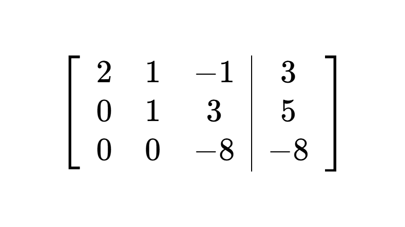
Gauss-Jordan Elimination
The Gauss-Jordan elimination method is a linear algebra algorithm designed to determine the solutions of a system of linear equations or to find the inverse of a given matrix. It is a direct extension of Gaussian elimination: instead of stopping once the matrix reaches an echelon structure (row echelon form) and using back-substitution, the reduction process continues transforming the matrix until each variable is completely isolated.
To apply this algorithm to a linear system, we place the coefficients of the variables and the constant terms into an augmented matrix. For instance, consider a general system of three linear equations with three variables:
$$\begin{cases} a_{11}x + a_{12}y + a_{13}z = b_1 \\ a_{21}x + a_{22}y + a_{23}z = b_2 \\ a_{31}x + a_{32}y + a_{33}z = b_3 \end{cases}$$
We write the augmented matrix by separating the column of constants with a vertical bar:
$$\left[\begin{array}{ccc|c} a_{11} & a_{12} & a_{13} & b_1 \\ a_{21} & a_{22} & a_{23} & b_2 \\ a_{31} & a_{32} & a_{33} & b_3 \end{array}\right]$$
The core objective of the algorithm is to transform the coefficient submatrix into reduced row echelon form (commonly abbreviated as RREF). This configuration decouples the variables, allowing the numerical value of each solution to be read directly from the final column without performing back-substitution.
A matrix is in reduced row echelon form when it strictly satisfies four conditions:
- If there are any rows consisting entirely of zeros, they must be located at the bottom of the matrix.
- The first nonzero entry in each nonzero row (called the pivot or leading 1) must be strictly equal to 1.
- In consecutive nonzero rows, the pivot in the lower row appears strictly to the right of the pivot in the upper row.
- In each column containing a pivot, all other entries (both above and below the leading 1) are zeros.
To transform the augmented matrix into this form without altering the solution set of the original system, we successively apply three elementary row operations (EROs):
- Row swap: \(R_i \leftrightarrow R_j\). Interchange the positions of row \(i\) and row \(j\).
- Scalar multiplication: \(R_i \to k \cdot R_i\) (where \(k \neq 0\)). Multiply every entry in row \(i\) by a nonzero constant \(k\).
- Row addition: \(R_i \to R_i + k \cdot R_j\). Replace row \(i\) with the sum of itself and a scalar multiple of row \(j\).
The fundamental distinction from classical Gaussian elimination lies in two requirements: in standard Gaussian elimination, pivots do not need to equal 1, and row operations only need to produce zeros below each pivot before solving the system through back-substitution. In contrast, Gauss-Jordan elimination requires clearing entries both below and above every pivot and normalizing each pivot to 1, eliminating the need for any subsequent back-substitution steps.
Table of Contents
How to Apply the Algorithm Step by Step
There are two primary operational approaches to transforming an augmented matrix into reduced row echelon form. While both lead to the exact same mathematical solution, the sequence in which pivots are normalized significantly impacts calculation complexity during manual computations.
Optimal Workflow for Manual Calculations
The vast majority of algebraic errors during exams do not stem from a misunderstanding of the method, but from carrying fraction addition and subtraction across multiple consecutive steps. To prevent awkward denominators from appearing early on, it is often more practical to postpone dividing by the pivot values until the very last step, dividing the process into three consecutive phases:
- Phase 1 (Forward Elimination): Start at the first nonzero column and select a nonzero pivot (interchanging rows if necessary). Using row addition operations, create zeros below that pivot. Repeat this process from left to right across each remaining submatrix until the matrix reaches standard row echelon form.
- Phase 2 (Backward Elimination): Identify the pivot in the bottom-most nonzero row. Working from bottom to top and from right to left, use this pivot to generate zeros in all positions directly above it. Repeat this step for the pivots in the intermediate rows until each pivot position is isolated within its column.
- Phase 3 (Final Normalization): Divide each row by its respective pivot value (or multiply by its reciprocal). This step simultaneously scales every pivot to 1 without having had to manipulate fractions during any of the preceding elimination phases.
Canonical Workflow
In standard university textbooks and formal lecture courses, the algorithm is typically introduced in the reverse order regarding row scaling: before eliminating entries in a column, the entire row is immediately divided by the pivot value to force a leading 1. The sequence proceeds as follows:
- Phase 1 (Pivot Normalization): Identify the active row and column, select a nonzero entry, and divide the entire row by that value to create a leading 1.
- Phase 2 (Forward Elimination): Use this normalized row to create zeros in every entry located below the leading 1. Repeat these first two phases column by column until reaching the final nonzero row.
- Phase 3 (Backward Elimination): Starting from the bottom-most pivot and moving upward, eliminate all nonzero entries located above each leading 1.
In computational implementations, software libraries often clear entries above and below simultaneously as soon as each column pivot is normalized, removing the need for a separate backward pass.
However, during hand calculations, clearing above and below at the same time carries an additional drawback: it obscures early identification of the system type (consistent independent, consistent dependent, or inconsistent), a classification that can be detected immediately after finishing the forward phase in a staged workflow.
Step-by-Step Example
To illustrate how the Gauss-Jordan elimination algorithm operates in practice using the optimal workflow, let us solve the following system of 3 equations with 3 variables. In the worked examples section, we will also demonstrate the canonical workflow when course requirements mandate normalizing pivots from the start.
$$\begin{cases} 2x + y - z = 0 \\ 4x + 5y + z = 6 \\ -2x + y + 2z = 1 \end{cases}$$
We write the augmented matrix of the system by organizing the variable coefficients and the constant terms:
$$\left[\begin{array}{ccc|c} 2 & 1 & -1 & 0 \\ 4 & 5 & 1 & 6 \\ -2 & 1 & 2 & 1 \end{array}\right]$$
We begin Phase 1 (Forward Elimination) working in the first column. We choose the 2 in the first row as our pivot and clear the entries located below it.
First, we eliminate the 4 in row 2 by subtracting twice row 1: \(R_2 \to R_2 - 2R_1\).
$$\left[\begin{array}{ccc|c} 2 & 1 & -1 & 0 \\ 0 & 3 & 3 & 6 \\ -2 & 1 & 2 & 1 \end{array}\right]$$
Next, we eliminate the −2 in row 3 by adding row 1 directly to row 3: \(R_3 \to R_3 + R_1\).
$$\left[\begin{array}{ccc|c} 2 & 1 & -1 & 0 \\ 0 & 3 & 3 & 6 \\ 0 & 2 & 1 & 1 \end{array}\right]$$
Before advancing to the second column, notice that all entries in row 2 are divisible by 3. To simplify the numbers and streamline subsequent calculations, we divide row 2 by 3: \(R_2 \to \frac{1}{3}R_2\).
$$\left[\begin{array}{ccc|c} 2 & 1 & -1 & 0 \\ 0 & 1 & 1 & 2 \\ 0 & 2 & 1 & 1 \end{array}\right]$$
The second pivot is now the 1 in row 2. We eliminate the 2 below it in row 3 by subtracting twice row 2: \(R_3 \to R_3 - 2R_2\).
$$\left[\begin{array}{ccc|c} 2 & 1 & -1 & 0 \\ 0 & 1 & 1 & 2 \\ 0 & 0 & -1 & -3 \end{array}\right]$$
The matrix is now in row echelon form. In classical Gaussian elimination, back-substitution would begin here; however, we continue applying row operations to carry out full Gauss-Jordan reduction.
We proceed with Phase 2 (Backward Elimination) to eliminate the entries located above the pivots, moving from the bottom row upward. The third pivot is −1, located in row 3, column 3. We use it to produce zeros in column 3 of the upper rows.
To eliminate the 1 in row 2, we add row 3 directly to row 2: \(R_2 \to R_2 + R_3\).
$$\left[\begin{array}{ccc|c} 2 & 1 & -1 & 0 \\ 0 & 1 & 0 & -1 \\ 0 & 0 & -1 & -3 \end{array}\right]$$
To eliminate the −1 in row 1, we subtract row 3 from row 1: \(R_1 \to R_1 - R_3\).
$$\left[\begin{array}{ccc|c} 2 & 1 & 0 & 3 \\ 0 & 1 & 0 & -1 \\ 0 & 0 & -1 & -3 \end{array}\right]$$
Moving up to row 2, the pivot is 1. We use it to eliminate the 1 above it in row 1 by subtracting row 2 from row 1: \(R_1 \to R_1 - R_2\).
$$\left[\begin{array}{ccc|c} 2 & 0 & 0 & 4 \\ 0 & 1 & 0 & -1 \\ 0 & 0 & -1 & -3 \end{array}\right]$$
All off-pivot entries in each pivot column are now zero. We conclude with Phase 3 (Final Normalization), scaling the remaining pivots to 1 in a single step:
- Divide row 1 by 2: \(R_1 \to \frac{1}{2}R_1\).
- Divide row 3 by −1 (or multiply by −1): \(R_3 \to -R_3\).
$$\left[\begin{array}{ccc|c} 1 & 0 & 0 & 2 \\ 0 & 1 & 0 & -1 \\ 0 & 0 & 1 & 3 \end{array}\right]$$
The coefficient submatrix is now the identity matrix. Writing out the resulting linear equations demonstrates how the solution values are read directly:
$$\begin{cases} 1x + 0y + 0z = 2 \implies x = 2 \\ 0x + 1y + 0z = -1 \implies y = -1 \\ 0x + 0y + 1z = 3 \implies z = 3 \end{cases}$$
The system has a unique solution: \(x = 2\), \(y = -1\), \(z = 3\). It is classified as a consistent independent system. We verify the result by substituting these values into the original equations:
$$\begin{cases} 2(2) + (-1) - (3) = 4 - 1 - 3 = 0 \\ 4(2) + 5(-1) + (3) = 8 - 5 + 3 = 6 \\ -2(2) + (-1) + 2(3) = -4 - 1 + 6 = 1 \end{cases}$$
All three equalities hold true simultaneously, confirming the accuracy of the solution.
Types of Solutions in 3×3 Systems
When applying the Gauss-Jordan elimination method to a system of three equations with three variables, the reduced row echelon form immediately reveals the nature of the solution set. The three possible outcomes that can arise from row reduction are summarized below:
| System Type | Reduced Matrix Structure | Algebraic Interpretation | Geometric Interpretation (in R3) |
|---|---|---|---|
| Consistent and independent (unique solution) | $$\left[\begin{array}{ccc|c} 1 & 0 & 0 & d_1 \\ 0 & 1 & 0 & d_2 \\ 0 & 0 & 1 & d_3 \end{array}\right]$$ | Unique solution. Each variable is completely isolated with a fixed numerical value: \(x = d_1\), \(y = d_2\), \(z = d_3\). | The three planes represented by the equations intersect at a single common point in three-dimensional space. |
| Consistent and dependent (infinitely many solutions) | $$\left[\begin{array}{ccc|c} 1 & 0 & c_1 & d_1 \\ 0 & 1 & c_2 & d_2 \\ 0 & 0 & 0 & 0 \end{array}\right]$$ | Infinitely many solutions. At least one row of zeros appears, \([0 \; 0 \; 0 \mid 0]\), representing the true identity \(0 = 0\). The variable lacking a leading 1 serves as a free variable (parameter \(t\)). | The three planes coincide entirely or intersect along a common line in space. |
| Inconsistent (no solution) | $$\left[\begin{array}{ccc|c} 1 & * & * & * \\ 0 & 1 & * & * \\ 0 & 0 & 0 & d \end{array}\right] \\~ \\ \text{ with } d \neq 0$$ | No solution. An inconsistent row of the form \([0 \; 0 \; 0 \mid d]\) appears, corresponding to the contradiction \(0 = d\). | The three planes do not share any common point (for example, disjoint parallel planes or planes intersecting pairwise along distinct lines). |
In consistent dependent systems, the number of free variables (or degrees of freedom) equals the total number of variables minus the number of leading 1s (pivots). Each free variable is assigned a scalar parameter belonging to the real numbers (commonly \(r, s, t\)), allowing the solution set to be expressed in parametric form.
Note that if an inconsistent row of the form \([0 \; 0 \; 0 \mid d]\) with \(d \neq 0\) appears during forward elimination, the system is immediately diagnosed as inconsistent. There is no need to continue with backward elimination or pivot normalizations, as the system has no solution.
Worked Examples
Below, we solve several practice problems by applying the Gauss-Jordan elimination algorithm to systems and matrices of varying dimensions.
2×2 Systems of Linear Equations
Two-variable linear systems help establish the mechanics of the Gauss-Jordan method before moving to larger systems.
Example 1
Solve the following system of linear equations using the Gauss-Jordan elimination method:
$$\begin{cases} 2x + 4y = 10 \\ 3x - y = 1 \end{cases}$$
Solution
We write the augmented matrix representing the system:
$$\left[\begin{array}{cc|c} 2 & 4 & 10 \\ 3 & -1 & 1 \end{array}\right]$$
Following the canonical workflow, we normalize the pivot in column 1 immediately by dividing row 1 by 2. Because all coefficients in that row are even, this does not introduce fractions: \(R_1 \to \frac{1}{2}R_1\).
$$\left[\begin{array}{cc|c} 1 & 2 & 5 \\ 3 & -1 & 1 \end{array}\right]$$
With the leading 1 established in column 1, we eliminate the entry below it (the 3 in row 2) by subtracting 3 times row 1: \(R_2 \to R_2 - 3R_1\).
$$\left[\begin{array}{cc|c} 1 & 2 & 5 \\ 0 & -7 & -14 \end{array}\right]$$
Moving to the second column, we normalize the pivot by dividing row 2 by −7: \(R_2 \to -\frac{1}{7}R_2\).
$$\left[\begin{array}{cc|c} 1 & 2 & 5 \\ 0 & 1 & 2 \end{array}\right]$$
We finish row reduction with backward elimination: using the leading 1 in row 2, we clear the 2 directly above it by subtracting twice row 2 from row 1: \(R_1 \to R_1 - 2R_2\).
$$\left[\begin{array}{cc|c} 1 & 0 & 1 \\ 0 & 1 & 2 \end{array}\right]$$
The matrix is now in reduced row echelon form (RREF) with the identity matrix on the left. The solution is read directly from the right-hand column:
$$\begin{cases} x = 1 \\ y = 2 \end{cases}$$
The system has a unique solution and is classified as a consistent independent system. Checking the solution in the original equations:
$$\begin{cases} 2(1) + 4(2) = 2 + 8 = 10 \\ 3(1) - (2) = 3 - 2 = 1 \end{cases}$$
Both equations are satisfied.
Example 2
Solve the following linear system using Gauss-Jordan elimination:
$$\begin{cases} 2x + 5y = 3 \\ 4x + 3y = 1 \end{cases}$$
Solution
We write the augmented matrix:
$$\left[\begin{array}{cc|c} 2 & 5 & 3 \\ 4 & 3 & 1 \end{array}\right]$$
Dividing row 1 by 2 at the start would immediately introduce fractions (\(\frac{5}{2}\) and \(\frac{3}{2}\)). To avoid intermediate fraction arithmetic, we apply the optimal workflow: eliminate off-diagonal entries using integer combinations and postpone normalization to the final step.
We begin Phase 1 (Forward Elimination) with 2 as our pivot. We clear the 4 in row 2 by subtracting twice row 1: \(R_2 \to R_2 - 2R_1\).
$$\left[\begin{array}{cc|c} 2 & 5 & 3 \\ 0 & -7 & -5 \end{array}\right]$$
We begin Phase 2 (Backward Elimination). The second pivot is −7. To eliminate the 5 in row 1 without fractions, we use a cross-multiplication combination: multiply row 1 by 7 and add 5 times row 2: \(R_1 \to 7R_1 + 5R_2\).
Computing each entry:
- Column 1: \(7(2) + 5(0) = 14 + 0 = 14\)
- Column 2: \(7(5) + 5(-7) = 35 - 35 = 0\)
- Constant column: \(7(3) + 5(-5) = 21 - 25 = -4\)
Updating row 1:
$$\left[\begin{array}{cc|c} 14 & 0 & -4 \\ 0 & -7 & -5 \end{array}\right]$$
With the coefficient block diagonalized, we execute Phase 3 (Final Normalization) by dividing each row by its respective pivot:
- Divide row 1 by 14: \(R_1 \to \frac{1}{14}R_1\)
- Divide row 2 by −7: \(R_2 \to -\frac{1}{7}R_2\)
$$\left[\begin{array}{cc|c} 1 & 0 & -\frac{4}{14} \\\\ 0 & 1 & \frac{5}{7} \end{array}\right]$$
Reducing the fraction in row 1:
$$\left[\begin{array}{cc|c} 1 & 0 & -\frac{2}{7} \\\\ 0 & 1 & \frac{5}{7} \end{array}\right]$$
We obtain the unique solution directly:
$$x = -\dfrac{2}{7}, \quad y = \dfrac{5}{7}$$
This is a consistent independent system with fractional solutions. Verifying by substitution:
$$\begin{cases} 2\left(-\dfrac{2}{7}\right) + 5\left(\dfrac{5}{7}\right) = -\dfrac{4}{7} + \dfrac{25}{7} = \dfrac{21}{7} = 3 \\\\ 4\left(-\dfrac{2}{7}\right) + 3\left(\dfrac{5}{7}\right) = -\dfrac{8}{7} + \dfrac{15}{7} = \dfrac{7}{7} = 1 \end{cases}$$
Both constant terms match the original system.
Example 3
Solve the following linear system using the Gauss-Jordan elimination algorithm:
$$\begin{cases} 2x - 6y = 4 \\ -x + 3y = -2 \end{cases}$$
Solution
We write the augmented matrix:
$$\left[\begin{array}{cc|c} 2 & -6 & 4 \\ -1 & 3 & -2 \end{array}\right]$$
All coefficients in row 1 are even, so we divide row 1 by 2 to obtain a leading 1: \(R_1 \to \frac{1}{2}R_1\).
$$\left[\begin{array}{cc|c} 1 & -3 & 2 \\ -1 & 3 & -2 \end{array}\right]$$
To eliminate the −1 in row 2, we add row 1 to row 2: \(R_2 \to R_2 + R_1\).
$$\left[\begin{array}{cc|c} 1 & -3 & 2 \\ 0 & 0 & 0 \end{array}\right]$$
The second row becomes entirely zeros, representing the true identity \(0 = 0\). This confirms that the second equation was a linear multiple of the first and provided no additional constraints.
The matrix is already in reduced row echelon form. Analyzing the columns:
- Column 1 contains a leading 1 corresponding to the basic variable x.
- Column 2 does not contain a pivot, making y a free variable.
We assign the free variable a real parameter \(t \in \mathbb{R}\):
$$y = t$$
Expressing row 1 in equation form to solve for x in terms of \(t\):
$$x - 3y = 2 \implies x = 2 + 3t$$
The system has infinitely many solutions and is classified as a consistent dependent system with one degree of freedom. The solution set is expressed as:
$$\text{Solution} = \left\{(2 + 3t, \; t) \mid t \in \mathbb{R}\right\}$$
3×3 Systems of Linear Equations
Systems of three linear equations in three variables are the most common format in exams. The following examples address strategic row swapping, dependent systems, and inconsistency.
Example 4
Solve the following system of linear equations using Gauss-Jordan elimination:
$$\begin{cases} 3x + y - z = -2 \\ x - 2y + z = 8 \\ 2x + 3y + z = -1 \end{cases}$$
Solution
We construct the augmented matrix:
$$\left[\begin{array}{ccc|c} 3 & 1 & -1 & -2 \\ 1 & -2 & 1 & 8 \\ 2 & 3 & 1 & -1 \end{array}\right]$$
Because row 2 already has a 1 in the first column, we interchange row 1 and row 2 to obtain an immediate leading 1 without division: \(R_1 \leftrightarrow R_2\).
$$\left[\begin{array}{ccc|c} 1 & -2 & 1 & 8 \\ 3 & 1 & -1 & -2 \\ 2 & 3 & 1 & -1 \end{array}\right]$$
We perform forward elimination to clear the entries below the leading 1:
- Subtract 3 times row 1 from row 2: \(R_2 \to R_2 - 3R_1\).
- Subtract 2 times row 1 from row 3: \(R_3 \to R_3 - 2R_1\).
$$\left[\begin{array}{ccc|c} 1 & -2 & 1 & 8 \\ 0 & 7 & -4 & -26 \\ 0 & 7 & -1 & -17 \end{array}\right]$$
In the second column, row 3 has the same entry (7) as row 2. We eliminate that entry by subtracting row 2 from row 3: \(R_3 \to R_3 - R_2\).
$$\left[\begin{array}{ccc|c} 1 & -2 & 1 & 8 \\ 0 & 7 & -4 & -26 \\ 0 & 0 & 3 & 9 \end{array}\right]$$
All entries in row 3 are multiples of 3; we divide row 3 by 3: \(R_3 \to \frac{1}{3}R_3\).
$$\left[\begin{array}{ccc|c} 1 & -2 & 1 & 8 \\ 0 & 7 & -4 & -26 \\ 0 & 0 & 1 & 3 \end{array}\right]$$
We begin the backward elimination phase using the 1 in row 3 to eliminate entries in column 3 above it:
- Add 4 times row 3 to row 2: \(R_2 \to R_2 + 4R_3\).
- Subtract row 3 from row 1: \(R_1 \to R_1 - R_3\).
$$\left[\begin{array}{ccc|c} 1 & -2 & 0 & 5 \\ 0 & 7 & 0 & -14 \\ 0 & 0 & 1 & 3 \end{array}\right]$$
Divide row 2 by 7: \(R_2 \to \frac{1}{7}R_2\).
$$\left[\begin{array}{ccc|c} 1 & -2 & 0 & 5 \\ 0 & 1 & 0 & -2 \\ 0 & 0 & 1 & 3 \end{array}\right]$$
Finally, clear the −2 in row 1 by adding twice row 2: \(R_1 \to R_1 + 2R_2\).
$$\left[\begin{array}{ccc|c} 1 & 0 & 0 & 1 \\ 0 & 1 & 0 & -2 \\ 0 & 0 & 1 & 3 \end{array}\right]$$
The coefficient matrix is now the identity matrix, giving the solution directly:
$$x = 1, \quad y = -2, \quad z = 3$$
The system is consistent and independent.
Resource: If you are solving practice problems and want to check your results, you can use our free tool:
Example 5
Find the solutions of the following linear system using Gauss-Jordan row reduction:
$$\begin{cases} 2x - 3z = 7 \\ x + 2y + z = 3 \\ 3x - 4y = 2 \end{cases}$$
Solution
When setting up the augmented matrix, place a 0 in positions where a variable is missing from an equation:
$$\left[\begin{array}{ccc|c} 2 & 0 & -3 & 7 \\ 1 & 2 & 1 & 3 \\ 3 & -4 & 0 & 2 \end{array}\right]$$
Swap row 1 with row 2 to place a 1 in the upper-left pivot position: \(R_1 \leftrightarrow R_2\).
$$\left[\begin{array}{ccc|c} 1 & 2 & 1 & 3 \\ 2 & 0 & -3 & 7 \\ 3 & -4 & 0 & 2 \end{array}\right]$$
Clear entries below the pivot in column 1:
- Subtract twice row 1 from row 2: \(R_2 \to R_2 - 2R_1\).
- Subtract 3 times row 1 from row 3: \(R_3 \to R_3 - 3R_1\).
$$\left[\begin{array}{ccc|c} 1 & 2 & 1 & 3 \\ 0 & -4 & -5 & 1 \\ 0 & -10 & -3 & -7 \end{array}\right]$$
To eliminate −10 in row 3 without fractions, use a cross-multiplication combination: replace row 3 with twice row 3 minus 5 times row 2: \(R_3 \to 2R_3 - 5R_2\).
Computing row 3 entries:
- Column 2: \(2(-10) - 5(-4) = -20 + 20 = 0\)
- Column 3: \(2(-3) - 5(-5) = -6 + 25 = 19\)
- Constant column: \(2(-7) - 5(1) = -14 - 5 = -19\)
Updating the matrix:
$$\left[\begin{array}{ccc|c} 1 & 2 & 1 & 3 \\ 0 & -4 & -5 & 1 \\ 0 & 0 & 19 & -19 \end{array}\right]$$
Divide row 3 by 19: \(R_3 \to \frac{1}{19}R_3\).
$$\left[\begin{array}{ccc|c} 1 & 2 & 1 & 3 \\ 0 & -4 & -5 & 1 \\ 0 & 0 & 1 & -1 \end{array}\right]$$
Begin backward elimination using the pivot in row 3 to clear column 3:
- Add 5 times row 3 to row 2: \(R_2 \to R_2 + 5R_3\).
- Subtract row 3 from row 1: \(R_1 \to R_1 - R_3\).
$$\left[\begin{array}{ccc|c} 1 & 2 & 0 & 4 \\ 0 & -4 & 0 & -4 \\ 0 & 0 & 1 & -1 \end{array}\right]$$
Divide row 2 by −4 to normalize its pivot: \(R_2 \to -\frac{1}{4}R_2\).
$$\left[\begin{array}{ccc|c} 1 & 2 & 0 & 4 \\ 0 & 1 & 0 & 1 \\ 0 & 0 & 1 & -1 \end{array}\right]$$
Finally, clear the 2 in row 1 by subtracting twice row 2: \(R_1 \to R_1 - 2R_2\).
$$\left[\begin{array}{ccc|c} 1 & 0 & 0 & 2 \\ 0 & 1 & 0 & 1 \\ 0 & 0 & 1 & -1 \end{array}\right]$$
The system is consistent and independent, with the unique solution:
$$x = 2, \quad y = 1, \quad z = -1$$
Example 6
Determine the solution of the following linear system containing fractional coefficients:
$$\begin{cases} \dfrac{x}{2} + \dfrac{y}{3} - \dfrac{z}{6} = 1 \\[2ex] x - \dfrac{y}{2} + z = \dfrac{7}{2} \\[2ex] \dfrac{x}{4} + y - \dfrac{z}{2} = \dfrac{1}{2} \end{cases}$$
Solution
Instead of building a matrix with fractions, clear denominators beforehand by multiplying each equation by the least common multiple (LCM) of its denominators:
- Equation 1: Multiply by \(\text{LCM}(2, 3, 6) = 6 \implies 3x + 2y - z = 6\).
- Equation 2: Multiply by \(\text{LCM}(1, 2) = 2 \implies 2x - y + 2z = 7\).
- Equation 3: Multiply by \(\text{LCM}(4, 1, 2) = 4 \implies x + 4y - 2z = 2\).
Using the integer equations, set up the augmented matrix:
$$\left[\begin{array}{ccc|c} 3 & 2 & -1 & 6 \\ 2 & -1 & 2 & 7 \\ 1 & 4 & -2 & 2 \end{array}\right]$$
Swap row 1 and row 3 to position the 1 as the pivot: \(R_1 \leftrightarrow R_3\).
$$\left[\begin{array}{ccc|c} 1 & 4 & -2 & 2 \\ 2 & -1 & 2 & 7 \\ 3 & 2 & -1 & 6 \end{array}\right]$$
Eliminate the entries below the pivot in column 1:
- Subtract twice row 1 from row 2: \(R_2 \to R_2 - 2R_1\).
- Subtract 3 times row 1 from row 3: \(R_3 \to R_3 - 3R_1\).
$$\left[\begin{array}{ccc|c} 1 & 4 & -2 & 2 \\ 0 & -9 & 6 & 3 \\ 0 & -10 & 5 & 0 \end{array}\right]$$
Both rows 2 and 3 can be simplified by dividing out common factors:
- Divide row 2 by −3: \(R_2 \to -\frac{1}{3}R_2\).
- Divide row 3 by −5: \(R_3 \to -\frac{1}{5}R_3\).
$$\left[\begin{array}{ccc|c} 1 & 4 & -2 & 2 \\ 0 & 3 & -2 & -1 \\ 0 & 2 & -1 & 0 \end{array}\right]$$
To eliminate the 2 in row 3 without fractions, subtract twice row 2 from 3 times row 3: \(R_3 \to 3R_3 - 2R_2\).
$$\left[\begin{array}{ccc|c} 1 & 4 & -2 & 2 \\ 0 & 3 & -2 & -1 \\ 0 & 0 & 1 & 2 \end{array}\right]$$
With the matrix in row echelon form, begin backward elimination using the pivot in row 3:
- Add twice row 3 to row 2: \(R_2 \to R_2 + 2R_3\).
- Add twice row 3 to row 1: \(R_1 \to R_1 + 2R_3\).
$$\left[\begin{array}{ccc|c} 1 & 4 & 0 & 6 \\ 0 & 3 & 0 & 3 \\ 0 & 0 & 1 & 2 \end{array}\right]$$
Divide row 2 by 3: \(R_2 \to \frac{1}{3}R_2\).
$$\left[\begin{array}{ccc|c} 1 & 4 & 0 & 6 \\ 0 & 1 & 0 & 1 \\ 0 & 0 & 1 & 2 \end{array}\right]$$
Subtract 4 times row 2 from row 1: \(R_1 \to R_1 - 4R_2\).
$$\left[\begin{array}{ccc|c} 1 & 0 & 0 & 2 \\ 0 & 1 & 0 & 1 \\ 0 & 0 & 1 & 2 \end{array}\right]$$
The unique solution is:
$$x = 2, \quad y = 1, \quad z = 2$$
Example 7
Solve the following linear system using Gauss-Jordan matrix elimination:
$$\begin{cases} 2x + 2y + z = 0 \\ 4x - 2y - z = 3 \\ 2x + 4y - 3z = -11 \end{cases}$$
Solution
We write the augmented matrix:
$$\left[\begin{array}{ccc|c} 2 & 2 & 1 & 0 \\ 4 & -2 & -1 & 3 \\ 2 & 4 & -3 & -11 \end{array}\right]$$
We begin forward elimination taking the 2 in row 1 as our pivot:
- Subtract twice row 1 from row 2: \(R_2 \to R_2 - 2R_1\).
- Subtract row 1 from row 3: \(R_3 \to R_3 - R_1\).
$$\left[\begin{array}{ccc|c} 2 & 2 & 1 & 0 \\ 0 & -6 & -3 & 3 \\ 0 & 2 & -4 & -11 \end{array}\right]$$
Divide row 2 by −3: \(R_2 \to -\frac{1}{3}R_2\).
$$\left[\begin{array}{ccc|c} 2 & 2 & 1 & 0 \\ 0 & 2 & 1 & -1 \\ 0 & 2 & -4 & -11 \end{array}\right]$$
Eliminate the 2 in row 3 by subtracting row 2 from row 3: \(R_3 \to R_3 - R_2\).
$$\left[\begin{array}{ccc|c} 2 & 2 & 1 & 0 \\ 0 & 2 & 1 & -1 \\ 0 & 0 & -5 & -10 \end{array}\right]$$
Divide row 3 by −5: \(R_3 \to -\frac{1}{5}R_3\).
$$\left[\begin{array}{ccc|c} 2 & 2 & 1 & 0 \\ 0 & 2 & 1 & -1 \\ 0 & 0 & 1 & 2 \end{array}\right]$$
Proceed with backward elimination using the pivot in row 3:
- Subtract row 3 from row 2: \(R_2 \to R_2 - R_3\).
- Subtract row 3 from row 1: \(R_1 \to R_1 - R_3\).
$$\left[\begin{array}{ccc|c} 2 & 2 & 0 & -2 \\ 0 & 2 & 0 & -3 \\ 0 & 0 & 1 & 2 \end{array}\right]$$
Clear the 2 in row 1 by subtracting row 2: \(R_1 \to R_1 - R_2\).
$$\left[\begin{array}{ccc|c} 2 & 0 & 0 & 1 \\ 0 & 2 & 0 & -3 \\ 0 & 0 & 1 & 2 \end{array}\right]$$
Now that the matrix is diagonalized, normalize rows 1 and 2 by dividing each by 2:
- \(R_1 \to \frac{1}{2}R_1\)
- \(R_2 \to \frac{1}{2}R_2\)
$$\left[\begin{array}{ccc|c} 1 & 0 & 0 & \frac{1}{2} \\\\ 0 & 1 & 0 & -\frac{3}{2} \\\\ 0 & 0 & 1 & 2 \end{array}\right]$$
Fractional values appear cleanly in the final step without cumbersome intermediate calculations:
$$x = \dfrac{1}{2}, \quad y = -\dfrac{3}{2}, \quad z = 2$$
Example 8
Analyze and solve the following linear system using Gauss-Jordan elimination:
$$\begin{cases} x - y + 2z = 3 \\ 2x + y + z = 3 \\ x + 2y - z = 0 \end{cases}$$
Solution
We write the augmented matrix:
$$\left[\begin{array}{ccc|c} 1 & -1 & 2 & 3 \\ 2 & 1 & 1 & 3 \\ 1 & 2 & -1 & 0 \end{array}\right]$$
The first pivot is already 1. Eliminate the entries beneath it:
- Subtract twice row 1 from row 2: \(R_2 \to R_2 - 2R_1\).
- Subtract row 1 from row 3: \(R_3 \to R_3 - R_1\).
$$\left[\begin{array}{ccc|c} 1 & -1 & 2 & 3 \\ 0 & 3 & -3 & -3 \\ 0 & 3 & -3 & -3 \end{array}\right]$$
Divide row 2 by 3: \(R_2 \to \frac{1}{3}R_2\).
$$\left[\begin{array}{ccc|c} 1 & -1 & 2 & 3 \\ 0 & 1 & -1 & -1 \\ 0 & 3 & -3 & -3 \end{array}\right]$$
Subtract 3 times row 2 from row 3: \(R_3 \to R_3 - 3R_2\).
$$\left[\begin{array}{ccc|c} 1 & -1 & 2 & 3 \\ 0 & 1 & -1 & -1 \\ 0 & 0 & 0 & 0 \end{array}\right]$$
Row 3 becomes all zeros (\(0 = 0\)). While there is no third pivot, we must complete backward elimination on the nonzero rows: eliminate the −1 in row 1 by adding row 2: \(R_1 \to R_1 + R_2\).
$$\left[\begin{array}{ccc|c} 1 & 0 & 1 & 2 \\ 0 & 1 & -1 & -1 \\ 0 & 0 & 0 & 0 \end{array}\right]$$
The matrix is now in reduced row echelon form (RREF):
- Columns 1 and 2 contain leading 1s corresponding to basic variables x and y.
- Column 3 lacks a pivot, making z a free variable.
Assign parameter \(t \in \mathbb{R}\) to the free variable:
$$z = t$$
Express basic variables in terms of the parameter:
$$\begin{cases} x + z = 2 \implies x = 2 - t \\ y - z = -1 \implies y = -1 + t \end{cases}$$
The system is consistent and dependent with one degree of freedom. The solution set is:
$$\text{Solution} = \left\{(2 - t, \; -1 + t, \; t) \mid t \in \mathbb{R}\right\}$$
Example 9
Solve and classify the following linear system:
$$\begin{cases} x + 2y - z = 2 \\ 2x - y + 3z = 1 \\ 3x + y + 2z = 5 \end{cases}$$
Solution
We write the augmented matrix:
$$\left[\begin{array}{ccc|c} 1 & 2 & -1 & 2 \\ 2 & -1 & 3 & 1 \\ 3 & 1 & 2 & 5 \end{array}\right]$$
Clear entries in column 1 below the pivot:
- Subtract twice row 1 from row 2: \(R_2 \to R_2 - 2R_1\).
- Subtract 3 times row 1 from row 3: \(R_3 \to R_3 - 3R_1\).
$$\left[\begin{array}{ccc|c} 1 & 2 & -1 & 2 \\ 0 & -5 & 5 & -3 \\ 0 & -5 & 5 & -1 \end{array}\right]$$
Eliminate the coefficient in row 3, column 2 by subtracting row 2 from row 3: \(R_3 \to R_3 - R_2\).
$$\left[\begin{array}{ccc|c} 1 & 2 & -1 & 2 \\ 0 & -5 & 5 & -3 \\ 0 & 0 & 0 & 2 \end{array}\right]$$
Examining row 3 reveals the form \([0 \; 0 \; 0 \mid 2]\), which translates to the equation:
$$0x + 0y + 0z = 2 \implies 0 = 2$$
This is a contradiction that cannot be satisfied by any choice of variables. Therefore, there is no need to perform backward elimination or normalizations: the system has no solution and is classified as inconsistent.
To systematically organize manual calculations and reduce arithmetic mistakes during Gauss-Jordan elimination, consider the following practical strategies:
- Clear denominators before setting up the matrix: If a linear system contains fractional coefficients, multiply each equation by the least common multiple of its denominators to work strictly with integers.
- Identify and align zero coefficients: If an equation is missing a variable, place an explicit zero in the corresponding column to preserve alignment and avoid an unnecessary elimination step.
- Prioritize unit pivots through row interchanges: Before forcing divisions that create fractions, check whether any lower row has a 1 or −1 in that column to perform a row swap (\(R_i \leftrightarrow R_j\)).
- Scale down rows with common divisors: If all entries in a row share a common factor following an elementary row operation, divide the entire row by that scalar to keep values small.
- Use integer cross-multiplication combinations: When a pivot does not divide the target entry evenly, apply linear combinations of the form \(R_i \to a \cdot R_i - b \cdot R_j\), postponing pivot division until the final step.
Rectangular and Higher-Order Systems
The Gauss-Jordan elimination algorithm maintains the exact same operational structure regardless of the number of rows or columns. Below, we examine systems with unequal numbers of equations and variables, higher-order systems, and standalone matrix reduction.
Example 10
Solve the following linear system using Gauss-Jordan elimination:
$$\begin{cases} x + 2y - z + 3w = 4 \\ 2x + 4y - z + 5w = 7 \end{cases}$$
Solution
We write the augmented matrix for this system of two equations with four variables:
$$\left[\begin{array}{cccc|c} 1 & 2 & -1 & 3 & 4 \\ 2 & 4 & -1 & 5 & 7 \end{array}\right]$$
The first pivot is the 1 in row 1. Eliminate the entry below it by subtracting twice row 1 from row 2: \(R_2 \to R_2 - 2R_1\).
$$\left[\begin{array}{cccc|c} 1 & 2 & -1 & 3 & 4 \\ 0 & 0 & 1 & -1 & -1 \end{array}\right]$$
Notice that column 2 contains a zero in row 2, meaning the next pivot falls in column 3 with a value of 1. We proceed with backward elimination to clear the entry above this pivot: add row 2 to row 1: \(R_1 \to R_1 + R_2\).
$$\left[\begin{array}{cccc|c} 1 & 2 & 0 & 2 & 3 \\ 0 & 0 & 1 & -1 & -1 \end{array}\right]$$
The matrix is now in reduced row echelon form. Analyzing pivot positions:
- Columns 1 and 3 contain leading 1s; thus, x and z are basic (pivot) variables.
- Columns 2 and 4 do not contain pivots, making y and w free variables.
With 4 variables and 2 pivots, the system has \(4 - 2 = 2\) degrees of freedom. Assign real parameters \(r, s \in \mathbb{R}\) to the free variables:
$$y = r, \quad w = s$$
Express the basic variables from the equations:
$$\begin{cases} x + 2y + 2w = 3 \implies x = 3 - 2r - 2s \\ z - w = -1 \implies z = -1 + s \end{cases}$$
The system has infinitely many solutions and is classified as a consistent dependent system with two parameters. The solution set is:
$$\text{Solution} = \left\{(3 - 2r - 2s, \; r, \; -1 + s, \; s) \mid r, s \in \mathbb{R}\right\}$$
Example 11
Determine the solution set of the following linear system:
$$\begin{cases} x + 2y = 1 \\ 2x - y = 7 \\ 3x + y = 8 \end{cases}$$
Solution
We write the augmented matrix for this overdetermined system of three equations and two variables:
$$\left[\begin{array}{cc|c} 1 & 2 & 1 \\ 2 & -1 & 7 \\ 3 & 1 & 8 \end{array}\right]$$
The initial pivot is 1. Eliminate the entries below it in column 1:
- Subtract twice row 1 from row 2: \(R_2 \to R_2 - 2R_1\).
- Subtract 3 times row 1 from row 3: \(R_3 \to R_3 - 3R_1\).
$$\left[\begin{array}{cc|c} 1 & 2 & 1 \\ 0 & -5 & 5 \\ 0 & -5 & 5 \end{array}\right]$$
Divide row 2 by −5: \(R_2 \to -\frac{1}{5}R_2\).
$$\left[\begin{array}{cc|c} 1 & 2 & 1 \\ 0 & 1 & -1 \\ 0 & -5 & 5 \end{array}\right]$$
Clear the −5 in row 3 by adding 5 times row 2: \(R_3 \to R_3 + 5R_2\).
$$\left[\begin{array}{cc|c} 1 & 2 & 1 \\ 0 & 1 & -1 \\ 0 & 0 & 0 \end{array}\right]$$
Complete backward elimination by removing the 2 in row 1: subtract twice row 2 from row 1: \(R_1 \to R_1 - 2R_2\).
$$\left[\begin{array}{cc|c} 1 & 0 & 3 \\ 0 & 1 & -1 \\ 0 & 0 & 0 \end{array}\right]$$
The last row became all zeros (\(0 = 0\)), confirming that the third original equation was a linear combination of the first two and introduces no contradictions. Because both variables have leading 1s with no free variables remaining, the system has a unique solution and is classified as a consistent independent system:
$$x = 3, \quad y = -1$$
Example 12
Solve the following system of 4 linear equations in 4 variables:
$$\begin{cases} x + y + z + w = 5 \\ 2x - y + z - w = 2 \\ -x + 2y + 2z + w = 4 \\ 3x + y - z + 2w = 6 \end{cases}$$
Solution
We construct the 4×5 augmented matrix:
$$\left[\begin{array}{cccc|c} 1 & 1 & 1 & 1 & 5 \\ 2 & -1 & 1 & -1 & 2 \\ -1 & 2 & 2 & 1 & 4 \\ 3 & 1 & -1 & 2 & 6 \end{array}\right]$$
Clear entries below the leading 1 in column 1:
- \(R_2 \to R_2 - 2R_1\)
- \(R_3 \to R_3 + R_1\)
- \(R_4 \to R_4 - 3R_1\)
$$\left[\begin{array}{cccc|c} 1 & 1 & 1 & 1 & 5 \\ 0 & -3 & -1 & -3 & -8 \\ 0 & 3 & 3 & 2 & 9 \\ 0 & -2 & -4 & -1 & -9 \end{array}\right]$$
Work on column 2 by eliminating entries below row 2:
- Add row 2 to row 3: \(R_3 \to R_3 + R_2\).
- Subtract twice row 2 from 3 times row 4: \(R_4 \to 3R_4 - 2R_2\).
$$\left[\begin{array}{cccc|c} 1 & 1 & 1 & 1 & 5 \\ 0 & -3 & -1 & -3 & -8 \\ 0 & 0 & 2 & -1 & 1 \\ 0 & 0 & -10 & 3 & -11 \end{array}\right]$$
In column 3, use the 2 in row 3 to eliminate −10 by adding 5 times row 3 to row 4: \(R_4 \to R_4 + 5R_3\).
$$\left[\begin{array}{cccc|c} 1 & 1 & 1 & 1 & 5 \\ 0 & -3 & -1 & -3 & -8 \\ 0 & 0 & 2 & -1 & 1 \\ 0 & 0 & 0 & -2 & -6 \end{array}\right]$$
Normalize row 4 by dividing by −2: \(R_4 \to -\frac{1}{2}R_4\).
$$\left[\begin{array}{cccc|c} 1 & 1 & 1 & 1 & 5 \\ 0 & -3 & -1 & -3 & -8 \\ 0 & 0 & 2 & -1 & 1 \\ 0 & 0 & 0 & 1 & 3 \end{array}\right]$$
Begin backward elimination using the leading 1 in row 4 to clear column 4:
- \(R_3 \to R_3 + R_4\)
- \(R_2 \to R_2 + 3R_4\)
- \(R_1 \to R_1 - R_4\)
$$\left[\begin{array}{cccc|c} 1 & 1 & 1 & 0 & 2 \\ 0 & -3 & -1 & 0 & 1 \\ 0 & 0 & 2 & 0 & 4 \\ 0 & 0 & 0 & 1 & 3 \end{array}\right]$$
Divide row 3 by 2: \(R_3 \to \frac{1}{2}R_3\).
$$\left[\begin{array}{cccc|c} 1 & 1 & 1 & 0 & 2 \\ 0 & -3 & -1 & 0 & 1 \\ 0 & 0 & 1 & 0 & 2 \\ 0 & 0 & 0 & 1 & 3 \end{array}\right]$$
Use the pivot in row 3 to clear column 3 entries above it:
- Add row 3 to row 2: \(R_2 \to R_2 + R_3\).
- Subtract row 3 from row 1: \(R_1 \to R_1 - R_3\).
$$\left[\begin{array}{cccc|c} 1 & 1 & 0 & 0 & 0 \\ 0 & -3 & 0 & 0 & 3 \\ 0 & 0 & 1 & 0 & 2 \\ 0 & 0 & 0 & 1 & 3 \end{array}\right]$$
Divide row 2 by −3: \(R_2 \to -\frac{1}{3}R_2\).
$$\left[\begin{array}{cccc|c} 1 & 1 & 0 & 0 & 0 \\ 0 & 1 & 0 & 0 & -1 \\ 0 & 0 & 1 & 0 & 2 \\ 0 & 0 & 0 & 1 & 3 \end{array}\right]$$
Conclude by subtracting row 2 from row 1: \(R_1 \to R_1 - R_2\).
$$\left[\begin{array}{cccc|c} 1 & 0 & 0 & 0 & 1 \\ 0 & 1 & 0 & 0 & -1 \\ 0 & 0 & 1 & 0 & 2 \\ 0 & 0 & 0 & 1 & 3 \end{array}\right]$$
The system is consistent and independent, with values read directly:
$$x = 1, \quad y = -1, \quad z = 2, \quad w = 3$$
Example 13
Find the reduced row echelon form (RREF) of the following matrix:
$$A = \begin{pmatrix} 1 & -2 & 3 & 1 \\ 2 & -4 & 7 & 3 \\ -1 & 2 & -1 & 3 \end{pmatrix}$$
Solution
The first pivot is at position (1, 1) with value 1. Eliminate the entries below it in column 1:
- \(R_2 \to R_2 - 2R_1\)
- \(R_3 \to R_3 + R_1\)
$$\begin{pmatrix} 1 & -2 & 3 & 1 \\ 0 & 0 & 1 & 1 \\ 0 & 0 & 2 & 4 \end{pmatrix}$$
In column 2, all entries below row 1 are already zeros. Consequently, we move to column 3, where the pivot is the 1 in row 2. Eliminate the 2 below it by subtracting twice row 2 from row 3: \(R_3 \to R_3 - 2R_2\).
$$\begin{pmatrix} 1 & -2 & 3 & 1 \\ 0 & 0 & 1 & 1 \\ 0 & 0 & 0 & 2 \end{pmatrix}$$
Normalize the final pivot by dividing row 3 by 2: \(R_3 \to \frac{1}{2}R_3\).
$$\begin{pmatrix} 1 & -2 & 3 & 1 \\ 0 & 0 & 1 & 1 \\ 0 & 0 & 0 & 1 \end{pmatrix}$$
Perform backward elimination to clear entries above the pivot in column 4:
- Subtract row 3 from row 2: \(R_2 \to R_2 - R_3\).
- Subtract row 3 from row 1: \(R_1 \to R_1 - R_3\).
$$\begin{pmatrix} 1 & -2 & 3 & 0 \\ 0 & 0 & 1 & 0 \\ 0 & 0 & 0 & 1 \end{pmatrix}$$
Finally, use the pivot in column 3 to eliminate the 3 in row 1: \(R_1 \to R_1 - 3R_2\).
$$\begin{pmatrix} 1 & -2 & 0 & 0 \\ 0 & 0 & 1 & 0 \\ 0 & 0 & 0 & 1 \end{pmatrix}$$
The matrix is now in reduced row echelon form (RREF). The pivot columns are columns 1, 3, and 4, while column 2 has no leading 1.
Example 14
Given the following partitioned matrix formed by a coefficient matrix on the left and the identity matrix on the right, apply row operations until obtaining the identity matrix in the left block:
$$\left[\begin{array}{cc|cc} 2 & 5 & 1 & 0 \\ 1 & 3 & 0 & 1 \end{array}\right] $$
Solution
Swap rows to place a 1 in the top-left position: \(R_1 \leftrightarrow R_2\).
$$\left[\begin{array}{cc|cc} 1 & 3 & 0 & 1 \\ 2 & 5 & 1 & 0 \end{array}\right]$$
Eliminate the 2 in row 2 by subtracting twice row 1: \(R_2 \to R_2 - 2R_1\).
$$\left[\begin{array}{cc|cc} 1 & 3 & 0 & 1 \\ 0 & -1 & 1 & -2 \end{array}\right]$$
Multiply row 2 by −1 to make its pivot positive: \(R_2 \to -R_2\).
$$\left[\begin{array}{cc|cc} 1 & 3 & 0 & 1 \\ 0 & 1 & -1 & 2 \end{array}\right]$$
Eliminate the 3 in row 1 by subtracting 3 times row 2: \(R_1 \to R_1 - 3R_2\).
$$\left[\begin{array}{cc|cc} 1 & 0 & 3 & -5 \\ 0 & 1 & -1 & 2 \end{array}\right]$$
The left block has transformed into the identity matrix. The matrix obtained in the right block, \(\begin{pmatrix} 3 & -5 \\ -1 & 2 \end{pmatrix}\), represents the exact inverse matrix of the original matrix \(\begin{pmatrix} 2 & 5 \\ 1 & 3 \end{pmatrix}\). This technique is one of the most prominent applications of Gauss-Jordan elimination.
Applications of Gauss-Jordan Elimination
While the Gauss-Jordan elimination algorithm is primarily used to solve systems of linear equations, its ability to reduce a matrix completely to the identity matrix allows it to solve other fundamental matrix problems.
Finding the Inverse Matrix
In elementary algebra, solving an equation like \(2x = 6\) involves multiplying both sides by the multiplicative inverse of 2 (which is \(\frac{1}{2}\)), yielding \(x = 3\). In matrix algebra, a similar principle applies: a complete linear system can be expressed compactly as \(A \cdot X = B\), where \(A\) is the coefficient matrix, \(X\) is the variable vector, and \(B\) is the constant vector.
If we can determine a matrix called the inverse matrix (denoted as \(A^{-1}\)), we can multiply both sides of the equation to isolate the solution vector directly: \(X = A^{-1} \cdot B\). The Gauss-Jordan algorithm provides the standard procedure for computing this inverse without needing determinant formulas and adjugate matrices.
The procedure consists of placing the original matrix \(A\) on the left and the identity matrix \(I\) of the same size on the right, separated by a vertical bar. We then apply elementary row operations until the identity matrix appears on the left; when this occurs, the matrix that forms on the right is automatically the inverse matrix:
$$[A \mid I] \longrightarrow [I \mid A^{-1}]$$
If a row of zeros appears on the left side during row reduction, the matrix cannot be reduced to the identity matrix and is therefore singular (non-invertible).
To see how this process works in three dimensions, let us compute the inverse of the following \(3 \times 3\) matrix:
$$A = \begin{pmatrix} 1 & 0 & 2 \\ 2 & -1 & 3 \\ 4 & 1 & 8 \end{pmatrix}$$
We construct the augmented matrix by placing the 3×3 identity matrix on the right:
$$\left[\begin{array}{ccc|ccc} 1 & 0 & 2 & 1 & 0 & 0 \\ 2 & -1 & 3 & 0 & 1 & 0 \\ 4 & 1 & 8 & 0 & 0 & 1 \end{array}\right]$$
The first pivot is the 1 in the top-left position. Eliminate entries below it in column 1:
- Subtract twice row 1 from row 2: \(R_2 \to R_2 - 2R_1\).
- Subtract 4 times row 1 from row 3: \(R_3 \to R_3 - 4R_1\).
$$\left[\begin{array}{ccc|ccc} 1 & 0 & 2 & 1 & 0 & 0 \\ 0 & -1 & -1 & -2 & 1 & 0 \\ 0 & 1 & 0 & -4 & 0 & 1 \end{array}\right]$$
To obtain a positive 1 for our second pivot without changing signs entry by entry, swap row 2 and row 3: \(R_2 \leftrightarrow R_3\).
$$\left[\begin{array}{ccc|ccc} 1 & 0 & 2 & 1 & 0 & 0 \\ 0 & 1 & 0 & -4 & 0 & 1 \\ 0 & -1 & -1 & -2 & 1 & 0 \end{array}\right]$$
Eliminate the −1 in row 3, column 2 by adding row 2 to row 3: \(R_3 \to R_3 + R_2\).
$$\left[\begin{array}{ccc|ccc} 1 & 0 & 2 & 1 & 0 & 0 \\ 0 & 1 & 0 & -4 & 0 & 1 \\ 0 & 0 & -1 & -6 & 1 & 1 \end{array}\right]$$
Multiply row 3 by −1 to normalize the third pivot to 1: \(R_3 \to -R_3\).
$$\left[\begin{array}{ccc|ccc} 1 & 0 & 2 & 1 & 0 & 0 \\ 0 & 1 & 0 & -4 & 0 & 1 \\ 0 & 0 & 1 & 6 & -1 & -1 \end{array}\right]$$
Proceed with backward elimination to clear entries above this final pivot. Row 2 already has a zero in that column, so we only need to clear the 2 in row 1 by subtracting twice row 3: \(R_1 \to R_1 - 2R_3\).
$$\left[\begin{array}{ccc|ccc} 1 & 0 & 0 & -11 & 2 & 2 \\ 0 & 1 & 0 & -4 & 0 & 1 \\ 0 & 0 & 1 & 6 & -1 & -1 \end{array}\right]$$
Because the identity matrix is now on the left, the block on the right is the desired inverse matrix:
$$A^{-1} = \begin{pmatrix} -11 & 2 & 2 \\ -4 & 0 & 1 \\ 6 & -1 & -1 \end{pmatrix}$$
If we had a system with coefficient matrix \(A\) and any set of constants \(B\), multiplying \(A^{-1} \cdot B\) would provide the values of \(x\), \(y\), and \(z\) immediately.
Solving Multiple Systems Simultaneously
In engineering, economics, and physics, systems frequently arise where the coefficient matrix remains fixed while the constant terms (external inputs, forces, or measurements) vary over time.
Instead of solving the system from scratch each time the right-hand side changes, Gauss-Jordan reduction allows solving all cases simultaneously in a single pass. To do this, place the shared coefficient matrix on the left and append multiple constant columns on the right:
$$\left[\begin{array}{c|ccc} A & B_1 & B_2 & B_3 \end{array}\right] \longrightarrow \left[\begin{array}{c|ccc} I & X_1 & X_2 & X_3 \end{array}\right]$$
Once elementary row operations transform the left side into the identity matrix, each column on the right directly yields the unique solution vector for its corresponding system.
Other Applications and More Efficient Alternatives
In linear algebra courses, Gauss-Jordan elimination is sometimes mentioned for two additional tasks: finding matrix rank and calculating determinants. However, more efficient alternatives are typically preferred in practice:
- Finding Matrix Rank: The rank of a matrix equals the number of nonzero rows in its echelon form. To find the rank, completing the forward phase (classical Gaussian elimination to REF) is sufficient; performing backward elimination and pivot scaling does not change the number of nonzero rows and adds unnecessary steps.
- Calculating Determinants: While elementary row operations can be used to evaluate determinants, row swaps flip the determinant's sign and row scalings alter its magnitude. Tracking these scalar factors while forcing an identity matrix in Gauss-Jordan is tedious and error-prone. For determinant calculations, simple Gaussian elimination is preferred: once an upper triangular matrix is reached, the determinant is computed directly by multiplying the entries along the main diagonal.
Did you find this useful? Rate it!
0.0 / 5 — 0 votes

HOW TO CITE THIS ARTICLE
Machado, D. (2026, October 20). Gauss-Jordan Elimination. Flamath. https://en.flamath.com/gauss-jordan-elimination
Gaussian Elimination
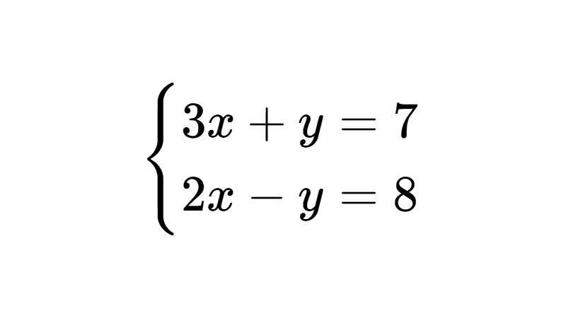
Solving Systems of Equations by Elimination
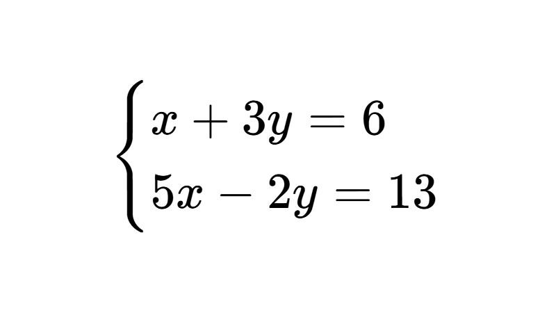
Solving Systems of Equations by Substitution
Leave a Reply
Related Articles