
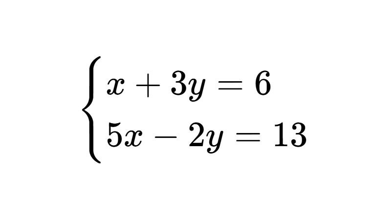
Systems of Linear Equations
A linear equation is an algebraic equation in which variables are only added or subtracted, multiplied by constant numbers, and raised to the first power. In its simplest two-variable form, it takes the standard structure ax + by = c.
A system of linear equations (or linear system) is a collection of two or more linear equations sharing the same variables that must be satisfied simultaneously. The core principle of a system is simultaneity: rather than looking for values that satisfy a single equation in isolation, we seek a set of numerical values that makes every equation in the system true at the same time.
To visualize this concept, consider the following system of two linear equations with two variables:
$$\begin{cases} x + y = 5 \\ 2x - y = 4 \end{cases}$$
Solving this system means finding a pair of numbers \((x, y)\) that satisfies both conditions simultaneously. If we choose \(x = 3\) and \(y = 2\), we can verify directly by substituting these values into each equation:
- First equation: substituting the values yields \(3 + 2 = 5\), which satisfies the equality.
- Second equation: evaluating gives \(2(3) - 2 = 6 - 2 = 4\), which also satisfies the equality.
Because the ordered pair \(x = 3\) and \(y = 2\) makes both equations true simultaneously, we say that \((3, 2)\) is a solution to the system. If an ordered pair satisfies one equation but fails in another, it is not a solution to the system.
Before exploring algebraic methods to find these solutions, it is essential to identify when an equation is no longer linear. Any algebraic operation that alters the first-degree exponent or multiplies variables together breaks the linearity of the model. Common non-linear expressions include:
- Exponents other than one: expressions such as \(x^2 + y = 9\), where at least one variable is raised to a power different from 1.
- Products of variables: equations such as \(xy + 3x = 10\), where two unknowns are multiplied together.
- Variables under radicals or in denominators: expressions like \(\sqrt{x} + y = 4\) or \(\frac{1}{x} + y = 2\).
- Transcendental functions: terms involving trigonometric, exponential, or logarithmic expressions applied to the variables, such as \(\sin(x) + y = 1\) or \(e^x - y = 0\).
Table of Contents
General Form and Notation of a Linear System
To analyze systems of any size, we first formalize the structure of an individual linear equation. In introductory algebra, we typically label variables using letters such as x, y, or z. When dealing with many variables, using numerical subscripts is far more practical: \(x_1, x_2, \dots, x_n\). A linear equation in \(n\) variables is written as:
$$a_1 x_1 + a_2 x_2 + \dots + a_n x_n = b$$
Each component of this equation serves a precise role in the algebraic model:
- Variables or unknowns (\(x_1, x_2, \dots, x_n\)): represent the unknown quantities whose numerical values we want to determine.
- Coefficients (\(a_1, a_2, \dots, a_n\)): fixed real numbers multiplying each variable. In mathematical notation, we write \(a_i \in \mathbb{R}\), where \(\in\) means "belongs to" and \(\mathbb{R}\) represents the set of real numbers.
- Constant term (\(b\)): a constant real number that does not multiply any variable, typically placed on the right-hand side of the equation.
When grouping \(m\) linear equations that share the same \(n\) variables, we obtain the general form of an \(m \times n\) linear system:
$$\begin{cases} a_{11}x_1 + a_{12}x_2 + \dots + a_{1n}x_n = b_1 \\ a_{21}x_1 + a_{22}x_2 + \dots + a_{2n}x_n = b_2 \\ \quad \vdots \\ a_{m1}x_1 + a_{m2}x_2 + \dots + a_{mn}x_n = b_m \end{cases}$$
The double subscript notation \(a_{ij}\) systematically tracks each coefficient. The first subscript (\(i\)) denotes the equation or row number, while the second subscript (\(j\)) indicates the variable it accompanies. For instance, coefficient \(a_{23}\) belongs to the second equation and multiplies variable \(x_3\).
A solution to this general system is an ordered list of \(n\) real numbers, known as an \(n\)-tuple and written as \((s_1, s_2, \dots, s_n)\), which verifies all \(m\) equations simultaneously upon substitution. The collection of all possible solutions admitted by the system is called the solution set.
A common misconception is assuming every linear system must have an equal number of equations and variables. The number of equations (\(m\)) and the number of variables (\(n\)) are completely independent, leading to three structural scenarios:
- Square systems (\(m = n\)): contain an equal number of equations and variables, such as a \(2 \times 2\) or \(3 \times 3\) system.
- Underdetermined systems (\(m < n\)): have fewer equations than variables (for example, a \(2 \times 3\) system with two equations and three variables). With fewer constraints than unknowns, these systems typically yield infinitely many solutions.
- Overdetermined systems (\(m > n\)): have more equations than variables (for example, a \(3 \times 2\) system with three equations and two variables). Imposing more constraints than variables often leads to contradictory or redundant equations.
Equivalent Systems and Elementary Operations
Two or more systems of linear equations are called equivalent if they share the exact same solution set, even when their individual equations have completely different numerical coefficients and appearances.
Every algebraic strategy for solving a linear system is built on this principle: rather than searching blindly for solutions, we transform the original system step by step into an equivalent system with a simpler structure until the values of the variables become explicit.
To ensure that these transformations preserve the exact solution set without adding extraneous solutions or removing valid ones, we apply three elementary operations:
- Interchanging two equations: swapping the order in which equations are listed does not alter the simultaneous conditions of the system.
- Multiplying an equation by a non-zero constant: scaling both sides of an equality by a non-zero real number preserves the original algebraic relationship.
- Adding a multiple of one equation to another: replacing an equation with the sum of itself and a multiple of another equation cancels variables while keeping the solution set intact.
To see how this works in practice, consider the following system of two equations with two variables:
$$\begin{cases} x + 2y = 8 \\ -x + y = 1 \end{cases}$$
Notice that variable \(x\) has opposite coefficients in both equations (1 in the first, -1 in the second). Applying the third elementary operation by adding the first equation directly to the second eliminates \(x\):
$$(x + 2y) + (-x + y) = 8 + 1 \implies 3y = 9$$
Replacing the original second equation with this result gives an equivalent system:
$$\begin{cases} x + 2y = 8 \\ 3y = 9 \end{cases}$$
This new system has the exact same solution set as the original, but solving it requires far less effort. From the second equation, we immediately deduce that \(y = 3\). Substituting this value into the first equation yields:
$$x + 2(3) = 8 \implies x + 6 = 8 \implies x = 2$$
The ordered pair \((2, 3)\) is the solution shared by both systems. This elementary process of progressive simplification forms the theoretical foundation for the algebraic elimination method and Gaussian elimination.
Types of Linear Systems by Number of Solutions
Every system of linear equations with real coefficients has exactly one of three possibilities regarding its solution set: exactly one unique solution, infinitely many solutions, or no solution.
In standard algebraic terminology, systems that have at least one solution are classified as consistent. If a consistent system has a single unique solution, it is called consistent and independent; if it has infinitely many solutions, it is called consistent and dependent. A system with no solution is classified as inconsistent.
To understand these three categories, it is helpful to look at their geometric interpretation. In the Cartesian plane (\(\mathbb{R}^2\)), each linear equation in two variables represents a straight line. Solving a \(2 \times 2\) system means finding the intersection of these lines: a single point where they cross, infinitely many points along a shared line if they coincide, or no points at all if they are parallel.
Similarly, in three-dimensional space (\(\mathbb{R}^3\)), each linear equation in three variables represents a flat plane, and the solution to the system corresponds to the intersection shared by these planes.
Consistent and Independent Systems (One Solution)
A consistent and independent system has exactly one unique solution satisfying all its equations simultaneously.
In the coordinate plane (\(\mathbb{R}^2\)), each equation describes a line, and a unique solution means the lines are intersecting lines that cross at a single point \((x, y)\). In three-dimensional space (\(\mathbb{R}^3\)), the equations describe planes that intersect at a single point \((x, y, z)\).
Example 1
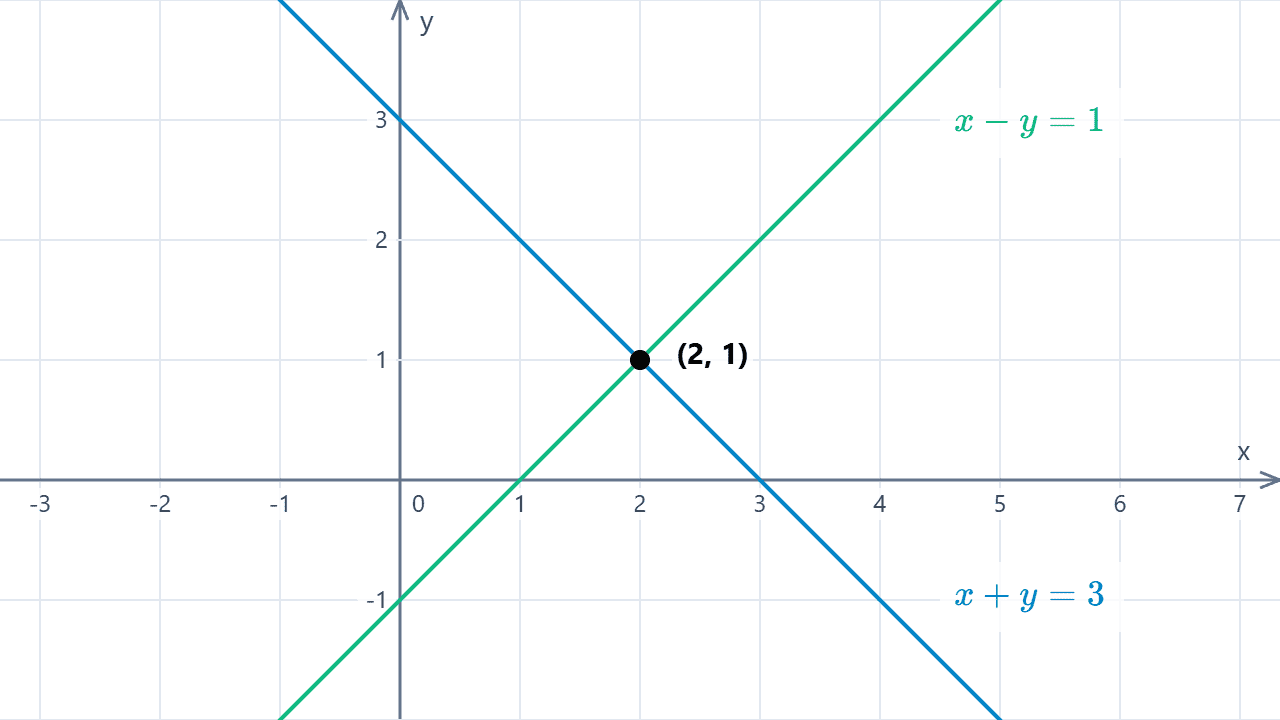
Consider the following system in the plane:
$$\begin{cases} x - y = 1 \\ x + y = 3 \end{cases}$$
Adding both equations together gives \(2x = 4\), which simplifies to \(x = 2\). Substituting this into the second equation yields \(2 + y = 3\), so \(y = 1\). The system has a unique solution given by the ordered pair \((2, 1)\).
Example 2
Consider this system of three equations with three variables:
$$\begin{cases} x + y + z = 6 \\ 2x - y + z = 3 \\ x + 2y - z = 2 \end{cases}$$
This system models three planes in three-dimensional space. Solving it algebraically reveals that the only ordered triple satisfying all three equations is \((x, y, z) = (1, 2, 3)\). Geometrically, all three planes intersect at that single point in space.
Example 3
Check the solution to the following overdetermined system of three equations with two variables:
$$\begin{cases} x + y = 4 \\ 2x - y = 2 \\ x + 2y = 6 \end{cases}$$
Although it is not a square system (having more equations than variables), the ordered pair \((x, y) = (2, 2)\) satisfies each equation:
- First equation: \(2 + 2 = 4\).
- Second equation: \(2(2) - 2 = 4 - 2 = 2\).
- Third equation: \(2 + 2(2) = 2 + 4 = 6\).
Because no other pair satisfies all three conditions simultaneously, this system is consistent and independent with the unique solution \((2, 2)\). In the coordinate plane, this represents three concurrent lines passing through the exact same point.
Consistent and Dependent Systems (Infinitely Many Solutions)
A consistent and dependent system has infinitely many solutions satisfying its equations.
When solving a dependent system algebraically, the process inevitably produces a trivial identity of the form 0 = 0. This result is not an error or contradiction; it indicates redundancy: one of the equations provides no new information and drops out, leaving one or more free variables that require parameterization.
Having infinitely many solutions does not mean any random combination of numbers works. The variables maintain a strict relationship. To express this infinite solution set, we leave one or more variables unconstrained as parameters (typically using letters such as t or s, where \(t, s \in \mathbb{R}\)). Expressing the remaining variables in terms of these parameters yields the parametric solution of the system.
In the Cartesian plane (\(\mathbb{R}^2\)), this occurs when the equations represent the exact same line: they are coincident lines, meaning every single point along the line is a valid solution. In three-dimensional space (\(\mathbb{R}^3\)), it occurs when planes intersect along a common line (one free parameter) or when all three planes coincide entirely (two free parameters).
Example 1
Consider the following system of two equations with two variables:
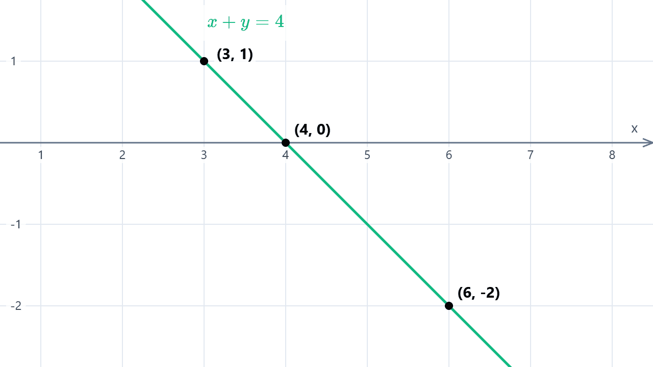
$$\begin{cases} x + y = 4 \\ 2x + 2y = 8 \end{cases}$$
Notice that the second equation is simply twice the first equation. Both equations represent the same line. To express the infinite solutions, solve for one variable, such as \(x = 4 - y\), and assign the free variable a parameter \(y = t\) (where \(t \in \mathbb{R}\)). The solution set in parametric form is:
$$(x, y) = (4 - t, t) \quad \text{for any } t \in \mathbb{R}$$
Every real number chosen for \(t\) produces a valid solution. If \(t = 0\), we get \((4, 0)\); if \(t = 1\), we get \((3, 1)\); if \(t = -2\), we get \((6, -2)\). All of these points lie on the line and verify both equations simultaneously.
Example 2
Consider an underdetermined \(2 \times 3\) system with more variables than equations:
$$\begin{cases} x + y + z = 5 \\ y - z = 1 \end{cases}$$
With three variables and only two independent equations, there are not enough constraints to identify a single point in space. From the second equation, we isolate \(y = 1 + z\). Substituting this into the first equation gives:
$$x + (1 + z) + z = 5 \implies x + 2z = 4 \implies x = 4 - 2z$$
Assigning the free parameter \(z = t\) (where \(t \in \mathbb{R}\)), the general solution in parametric form is:
$$(x, y, z) = (4 - 2t, 1 + t, t) \quad \text{for any } t \in \mathbb{R}$$
Geometrically, this represents two non-parallel planes in three dimensions intersecting along an infinite line, whose coordinates are mapped by the parameter \(t\).
Inconsistent Systems (No Solution)
An inconsistent system is a system that has no solution satisfying all equations simultaneously.
Algebraically, attempting to solve an inconsistent system leads to a mathematical contradiction of the form 0 = k, where k is a non-zero constant. Because no values of real variables can make a false statement like 0 = 3 true, the solution set is the empty set (denoted by \(\emptyset\)).
In the Cartesian plane (\(\mathbb{R}^2\)), an inconsistent system corresponds to parallel lines: they have identical slopes but different y-intercepts, meaning they never intersect. In three-dimensional space (\(\mathbb{R}^3\)), it represents planes that are parallel and distinct, or planes that intersect in pairs along distinct parallel lines without sharing any common line or point.
Example 1
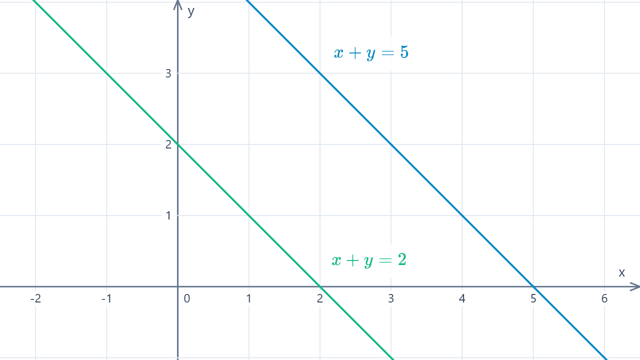
Consider the following system of two equations with two variables:
$$\begin{cases} x + y = 2 \\ x + y = 5 \end{cases}$$
Subtracting the first equation from the second eliminates both variables simultaneously:
$$(x + y) - (x + y) = 5 - 2 \implies 0 = 3$$
This statement is an obvious contradiction. No two numbers can sum to 2 and 5 at the same time. Therefore, the system has no solution and is classified as inconsistent.
Example 2
Consider a system of three equations with two variables in the plane:
$$\begin{cases} x - y = 1 \\ x + y = 3 \\ 2x + y = 8 \end{cases}$$
Solving the first two equations gives the unique intersection point \((x, y) = (2, 1)\). However, substituting this pair into the third equation gives \(2(2) + 1 = 5 \neq 8\). Although the lines intersect in pairs, all three lines do not meet at a single shared point, making the system inconsistent.
Comparison Table
The following table summarizes the classification of linear systems:
| System Classification | Number of Solutions | Algebraic Result | Geometric Meaning in \(\mathbb{R}^2\) |
|---|---|---|---|
| Consistent and Independent | One unique solution | Definite values for each variable: \((x, y)\) | Intersecting lines crossing at a single point |
| Consistent and Dependent | Infinitely many solutions | Identity: \(0 = 0\) (free parameters) | Coincident lines (same line) |
| Inconsistent | No solution | Contradiction: \(0 = k\) with \(k \neq 0\) | Parallel lines that never intersect |
This tripartite classification applies equally in higher dimensions (\(\mathbb{R}^n\) for \(n \ge 4\)). While we cannot visualize hyperplanes in four or more dimensions, the algebraic properties remain identical: any linear system, regardless of its size, has either exactly one solution, infinitely many solutions, or no solution.
Methods for Solving Systems of Linear Equations
There are multiple algebraic approaches to solve a system of linear equations. Choosing the most efficient method depends on the number of equations, the number of variables, and the coefficients involved.
While small \(2 \times 2\) systems are easily handled using graphing, substitution, or elimination, larger systems require systematic algorithmic techniques such as Gaussian elimination, Gauss-Jordan elimination, or matrix algebra.
Substitution Method
The substitution method involves solving for one variable in one equation and substituting that expression into the other equation. This reduces a two-variable system to a single linear equation in one unknown. Substitution is especially efficient when at least one variable has a coefficient of 1 or -1, as it isolates the variable without introducing intermediate fractions.
Note: When both equations already have the same variable isolated (such as \(y = 2x - 5\) and \(y = 5 - 3x\)), setting them equal to each other (\(2x - 5 = 5 - 3x\)) is simply a direct application of the substitution method.
Example
Solve the following system using substitution:
$$\begin{cases} x - 2y = 7 \\ 3x + y = 7 \end{cases}$$
Solve for \(x\) in the first equation:
$$x = 7 + 2y$$
Substitute this expression into the second equation in place of \(x\):
$$3(7 + 2y) + y = 7 \implies 21 + 6y + y = 7 \implies 7y = 7 - 21 \implies 7y = -14 \implies y = -2$$
Now find \(x\) by substituting \(y = -2\) back into our expression for \(x\):
$$x = 7 + 2(-2) \implies x = 7 - 4 \implies x = 3$$
The solution to the system is the ordered pair \((3, -2)\).
Elimination Method
The elimination method (also called the addition method) involves multiplying one or both equations by suitable constants so that the coefficients of one variable become opposites. Adding the two equations together eliminates that variable immediately. This is usually the cleanest method when variable coefficients are integers other than 1, preventing fractional expressions in early steps.
Example
Solve the following system using the elimination method:
$$\begin{cases} 2x + 3y = 1 \\ 5x - 2y = 12 \end{cases}$$
To eliminate variable \(y\), multiply the first equation by 2 and the second equation by 3 to create opposite coefficients of 6 and -6:
$$\begin{cases} 2 \cdot (2x + 3y = 1) \implies 4x + 6y = 2 \\ 3 \cdot (5x - 2y = 12) \implies 15x - 6y = 36 \end{cases}$$
Add the equations together to eliminate the \(y\) terms:
$$(4x + 15x) + (6y - 6y) = 2 + 36 \implies 19x = 38 \implies x = 2$$
Substitute \(x = 2\) into either original equation, such as the first:
$$2(2) + 3y = 1 \implies 4 + 3y = 1 \implies 3y = -3 \implies y = -1$$
The unique solution to the system is the ordered pair \((2, -1)\).
Graphing Method
The graphing method approaches the system geometrically in the Cartesian plane. Each linear equation is graphed as a straight line—usually by converting to slope-intercept form (\(y = mx + b\)) or plotting intercepts—and the solution is found by visually locating the point of intersection.
While graphing provides strong visual intuition, its precision is limited. If the intersection involves fractional or decimal coordinates (such as \(\frac{7}{13}\)), reading exact values off a grid is virtually impossible, making algebraic methods preferred for exact calculations. However, graphing is ideal for immediately identifying inconsistent systems (parallel lines) or dependent systems (coincident lines).
Example
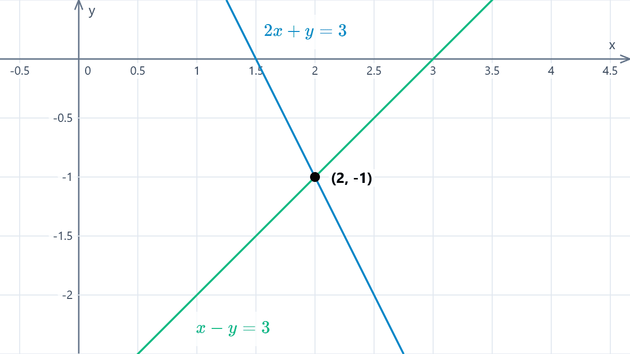
Find the intersection point of the following linear system graphically:
$$\begin{cases} x - y = 3 \\ 2x + y = 3 \end{cases}$$
Isolate \(y\) in each equation to identify the slope and y-intercept:
- First line: \(y = x - 3\) (slope \(m = 1\), y-intercept \(-3\))
- Second line: \(y = -2x + 3\) (slope \(m = -2\), y-intercept \(3\))
Plotting both lines reveals that they cross at a single point: \(x = 2\) and \(y = -1\). We verify algebraically that \(2 - (-1) = 3\) and \(2(2) + (-1) = 3\), confirming that \((2, -1)\) is the exact solution.
Gaussian Elimination
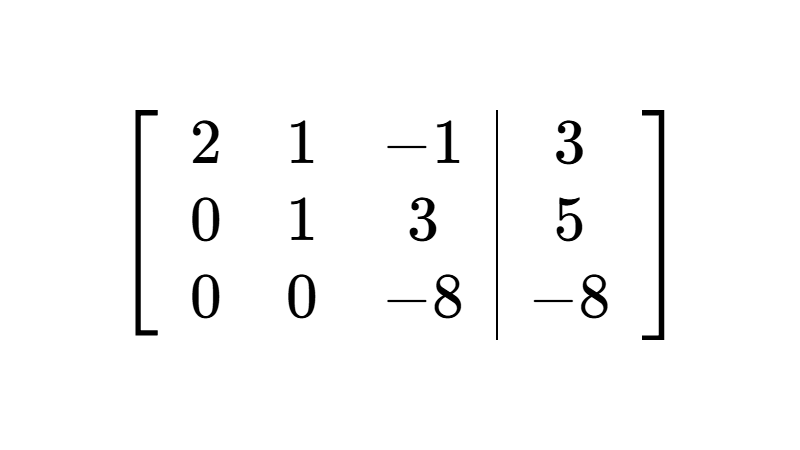
Gaussian elimination is a systematic algorithm designed to solve linear systems of any size. It transforms the system into an equivalent upper triangular system in row echelon form (REF), from which solutions are found using back-substitution. To streamline calculations, coefficients and constant terms are written in an augmented matrix.
For a standard \(3 \times 3\) system, the correspondence between equations and its augmented matrix is:
$$\begin{cases} a_{11}x + a_{12}y + a_{13}z = b_1 \\ a_{21}x + a_{22}y + a_{23}z = b_2 \\ a_{31}x + a_{32}y + a_{33}z = b_3 \end{cases} \quad \longrightarrow \quad \left[\begin{array}{ccc|c} a_{11} & a_{12} & a_{13} & b_1 \\ a_{21} & a_{22} & a_{23} & b_2 \\ a_{31} & a_{32} & a_{33} & b_3 \end{array}\right]$$
The elementary operations on equations correspond directly to three elementary row operations on matrices:
- Row swapping: \(R_i \leftrightarrow R_j\). Swaps row \(i\) with row \(j\).
- Scalar multiplication: \(R_i \to k \cdot R_i\) (where \(k \neq 0\)). Multiplies row \(i\) by non-zero constant \(k\).
- Row addition: \(R_i \to R_i + k \cdot R_j\). Adds a scalar multiple of row \(j\) to row \(i\).
The objective is to produce a matrix in row echelon form, which meets three criteria:
- Any rows consisting entirely of zeros are placed at the bottom of the matrix.
- The leading non-zero entry (the pivot) in each non-zero row is strictly to the right of the pivot in the row above it.
- All entries in a column below a pivot are zeros.
Example
Solve the following \(3 \times 3\) system using Gaussian elimination:
$$\begin{cases} x + 2y - z = 2 \\ 2x + 5y + z = 11 \\ -x - y + 3z = 4 \end{cases}$$
Set up the augmented matrix:
$$\left[\begin{array}{ccc|c} 1 & 2 & -1 & 2 \\ 2 & 5 & 1 & 11 \\ -1 & -1 & 3 & 4 \end{array}\right]$$
Using the pivot in the first column, create zeros underneath by applying \(R_2 \to R_2 - 2R_1\) and \(R_3 \to R_3 + R_1\):
$$\left[\begin{array}{ccc|c} 1 & 2 & -1 & 2 \\ 0 & 1 & 3 & 7 \\ 0 & 1 & 2 & 6 \end{array}\right]$$
Using the pivot in row 2, eliminate the entry below it by performing \(R_3 \to R_3 - R_2\):
$$\left[\begin{array}{ccc|c} 1 & 2 & -1 & 2 \\ 0 & 1 & 3 & 7 \\ 0 & 0 & -1 & -1 \end{array}\right]$$
The matrix is now in row echelon form. Rewrite the corresponding system to solve by back-substitution:
- From row 3: \(-z = -1 \implies z = 1\).
- From row 2: \(y + 3z = 7 \implies y + 3(1) = 7 \implies y = 4\).
- From row 1: \(x + 2y - z = 2 \implies x + 2(4) - 1 = 2 \implies x + 7 = 2 \implies x = -5\).
The unique solution is the ordered triple \((x, y, z) = (-5, 4, 1)\).
Gauss-Jordan Elimination
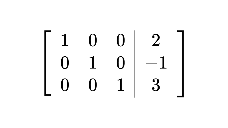
Gauss-Jordan elimination extends Gaussian elimination by continuing row operations to eliminate entries above each pivot as well as below. Normalizing all pivots to 1 transforms the augmented matrix into reduced row echelon form (RREF), where the final values of the variables can be read directly from the augmented column without back-substitution.
Example
Continue from the row echelon matrix obtained in the previous example:
$$\left[\begin{array}{ccc|c} 1 & 2 & -1 & 2 \\ 0 & 1 & 3 & 7 \\ 0 & 0 & -1 & -1 \end{array}\right]$$
Using the pivot in the third row (\(-1\)), clear the entries above it by applying \(R_2 \to R_2 + 3R_3\) and \(R_1 \to R_1 - R_3\):
$$\left[\begin{array}{ccc|c} 1 & 2 & 0 & 3 \\ 0 & 1 & 0 & 4 \\ 0 & 0 & -1 & -1 \end{array}\right]$$
Using the pivot in row 2 (\(1\)), eliminate the entry above it in row 1 by performing \(R_1 \to R_1 - 2R_2\):
$$\left[\begin{array}{ccc|c} 1 & 0 & 0 & -5 \\ 0 & 1 & 0 & 4 \\ 0 & 0 & -1 & -1 \end{array}\right]$$
Scale row 3 by multiplying by \(-1\) (\(R_3 \to -1 \cdot R_3\)) so all leading pivots equal 1:
$$\left[\begin{array}{ccc|c} 1 & 0 & 0 & -5 \\ 0 & 1 & 0 & 4 \\ 0 & 0 & 1 & 1 \end{array}\right]$$
The matrix is now in reduced row echelon form (RREF). The solution is read directly:
$$\begin{cases} 1x + 0y + 0z = -5 \implies x = -5 \\ 0x + 1y + 0z = 4 \implies y = 4 \\ 0x + 0y + 1z = 1 \implies z = 1 \end{cases}$$
The solution is confirmed as \((-5, 4, 1)\).
Cramer's Rule
Cramer's rule is an analytical method that solves a linear system using determinants. It requires two conditions: the system must be square (\(n \times n\)) and the determinant of the coefficient matrix (denoted \(\Delta\) or \(\det(A)\)) must be non-zero (\(\Delta \neq 0\)).
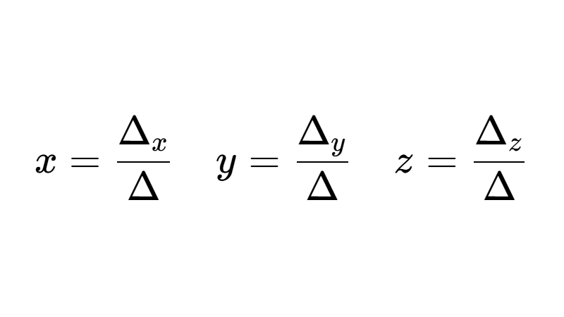
When these conditions are met, each variable is calculated by dividing a specific matrix determinant by the coefficient determinant:
$$x_i = \frac{\Delta_{x_i}}{\Delta}$$
The determinant \(\Delta_{x_i}\) is formed by replacing the \(i\)-th column of the coefficient matrix with the constant terms column vector.
Example
Solve the following system using Cramer's rule:
$$\begin{cases} 3x + 2y = 7 \\ 4x - 3y = -2 \end{cases}$$
First, calculate the determinant of the coefficient matrix \(\Delta\):
$$\Delta = \begin{vmatrix} 3 & 2 \\ 4 & -3 \end{vmatrix} = (3)(-3) - (2)(4) = -9 - 8 = -17$$
Since \(\Delta \neq 0\), the system is consistent and independent. To compute \(\Delta_x\), replace the first column (coefficients of \(x\)) with the constant terms 7 and -2:
$$\Delta_x = \begin{vmatrix} 7 & 2 \\ -2 & -3 \end{vmatrix} = (7)(-3) - (2)(-2) = -21 - (-4) = -21 + 4 = -17$$
Similarly, to compute \(\Delta_y\), replace the second column (coefficients of \(y\)) with the constant terms:
$$\Delta_y = \begin{vmatrix} 3 & 7 \\ 4 & -2 \end{vmatrix} = (3)(-2) - (7)(4) = -6 - 28 = -34$$
Finally, calculate the value of each variable:
$$x = \frac{\Delta_x}{\Delta} = \frac{-17}{-17} = 1$$
$$y = \frac{\Delta_y}{\Delta} = \frac{-34}{-17} = 2$$
The unique solution is the ordered pair \((1, 2)\).
Use the following comparison table to choose the best method for your problem:
| Method | Best Suited For | Key Advantages | Limitations |
|---|---|---|---|
| Substitution | \(2 \times 2\) systems with an easily isolated variable | Very fast when a coefficient is 1 or -1 | Leads to tedious fractions if no coefficient is 1 |
| Elimination | \(2 \times 2\) systems with non-unit integer coefficients | Avoids early fractional calculations | Requires finding suitable multipliers to cancel variables |
| Graphing | \(2 \times 2\) systems for qualitative visual analysis | Quickly visualizes whether lines intersect, coincide, or run parallel | Poor numerical precision for fractional or decimal solutions |
| Gaussian Elimination | \(3 \times 3\) systems or general \(m \times n\) systems | Universal algorithm applicable to any size or shape | Requires back-substitution after row echelon form is reached |
| Gauss-Jordan Elimination | \(3 \times 3\) or larger linear systems | Yields exact variable values directly from RREF | More row operations required to clear entries above pivots |
| Cramer's Rule | Small square systems (\(2 \times 2\) or \(3 \times 3\)) with \(\Delta \neq 0\) | Closed-form algebraic formula based on determinants | Inapplicable if \(\Delta = 0\) or if \(m \neq n\); computationally inefficient for \(n > 3\) |
Matrix Representation of a Linear System
In linear algebra, systems of linear equations are written compactly using matrix and vector notation. This converts a collection of simultaneous equations into a single matrix equation, enabling global theoretical analysis and efficient numerical computation.
Any general linear system of \(m\) equations with \(n\) variables can be represented in standard matrix form as Ax = b:
$$\begin{bmatrix} a_{11} & a_{12} & \dots & a_{1n} \\ a_{21} & a_{22} & \dots & a_{2n} \\ \vdots & \vdots & \ddots & \vdots \\ a_{m1} & a_{m2} & \dots & a_{mn} \end{bmatrix} \begin{bmatrix} x_1 \\ x_2 \\ \vdots \\ x_n \end{bmatrix} = \begin{bmatrix} b_1 \\ b_2 \\ \vdots \\ b_m \end{bmatrix}$$
This structure consists of three matrix components:
- Coefficient matrix (A): an \(m \times n\) matrix containing the numerical coefficients of the variables.
- Variable vector (x): an \(n \times 1\) column vector containing the unknown variables to be determined.
- Constant vector (b): an \(m \times 1\) column vector containing the constant terms from the right-hand side of each equation.
Applying standard matrix multiplication (multiplying each row of A by column vector x) reconstructs the original system of equations exactly.
Solving Using Inverse Matrices
When working with a square system where the number of equations equals the number of variables (\(n \times n\)), the matrix equation \(A\mathbf{x} = \mathbf{b}\) leads to an algebraic solution analogous to standard division. If the coefficient matrix A is invertible—which occurs whenever its determinant is non-zero (\(\det(A) \neq 0\))—there exists a unique inverse matrix \(A^{-1}\).
Multiplying both sides on the left by \(A^{-1}\) solves for the variable vector directly:
$$A\mathbf{x} = \mathbf{b} \implies A^{-1}(A\mathbf{x}) = A^{-1}\mathbf{b} \implies I\mathbf{x} = A^{-1}\mathbf{b} \implies \mathbf{x} = A^{-1}\mathbf{b}$$
Here, I is the identity matrix. This shows that the solution vector is obtained by multiplying the inverse matrix \(A^{-1}\) by the constant vector \(\mathbf{b}\). While foundational in theoretical mathematics, computing \(A^{-1}\) by hand is rarely practical for large systems, as finding an inverse matrix is computationally more expensive than Gaussian elimination.
Homogeneous Systems
A homogeneous system is a linear system in which all constant terms are equal to zero. In matrix form, it is written as Ax = 0, where 0 represents the zero vector.
A defining property of homogeneous systems is that they can never be inconsistent. They always have at least the trivial solution, where every variable is zero (\(x_1 = 0, x_2 = 0, \dots, x_n = 0\)). Therefore, only two possibilities exist for a homogeneous system:
- Only the trivial solution exists: the system is consistent and independent. For square systems, this occurs if and only if \(\det(A) \neq 0\).
- Non-trivial solutions exist (infinitely many solutions): the system is consistent and dependent. For square systems, this occurs when \(\det(A) = 0\). For rectangular systems with more variables than equations (\(n > m\)), infinitely many non-trivial solutions are mathematically guaranteed.
Real-World Applications and Linear Modeling
The practical value of linear systems lies in modeling real-world problems. In engineering, business, economics, and science, problems rarely arrive as pre-formulated equations; they appear as relationships and constraints expressed in everyday language. The process of translating verbal statements into mathematical equations is known as linear modeling.
To set up and solve word problems systematically, follow this three-step process:
- Identify and define variables: clearly determine which unknown quantities are requested, assign an algebraic variable to each, and specify their units of measurement (e.g., items, hours, dollars).
- Translate verbal constraints into equations: each statement or quantitative condition typically represents a balanced relationship, yielding one equation in the system.
- Solve and interpret the results in context: after calculating the numerical solution, verify that the answers satisfy the physical constraints of the problem (such as requiring non-negative quantities or whole numbers).
Example
A workshop produces two types of handcrafted lamps: classic and modern. A classic lamp requires 2 hours of assembly and 1 hour of painting. A modern lamp requires 3 hours of assembly and 2 hours of painting. If the workshop has 18 hours available for assembly and 11 hours for painting each week, how many lamps of each type should be produced to use all available hours?
Solution
First, define the variables:
- \(x\): number of classic lamps to produce.
- \(y\): number of modern lamps to produce.
- Both variables must be non-negative integers (\(x, y \ge 0\)).
Translate the problem constraints into equations:
- Assembly time constraint: \(x\) classic lamps take 2 hours each and \(y\) modern lamps take 3 hours each, totaling 18 hours: \(2x + 3y = 18\).
- Painting time constraint: \(x\) classic lamps take 1 hour each and \(y\) modern lamps take 2 hours each, totaling 11 hours: \(x + 2y = 11\).
This gives the following linear system:
$$\begin{cases} 2x + 3y = 18 \\ x + 2y = 11 \end{cases}$$
Solve by substitution by isolating \(x\) in the second equation:
$$x = 11 - 2y$$
Substitute this expression into the first equation:
$$2(11 - 2y) + 3y = 18 \implies 22 - 4y + 3y = 18 \implies 22 - y = 18 \implies -y = 18 - 22 \implies y = 4$$
Find \(x\) by substituting \(y = 4\) back into our expression for \(x\):
$$x = 11 - 2(4) \implies x = 11 - 8 \implies x = 3$$
Interpreting the solution in context: the workshop should produce 3 classic lamps and 4 modern lamps per week. Both values are positive integers that satisfy all hourly constraints.
Linear Systems Topics
Did you find this useful? Rate it!
0.0 / 5 — 0 votes

HOW TO CITE THIS ARTICLE
Machado, D. (2026, November 7). Systems of Linear Equations. Flamath. https://en.flamath.com/linear-systems
Cramer's Rule
Gauss-Jordan Elimination
Gaussian Elimination
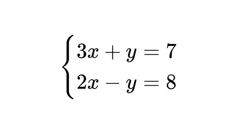
Solving Systems of Equations by Elimination
Solving Systems of Equations by Substitution
Leave a Reply
Related Articles