Constructive Dilemma

The constructive dilemma is a fundamental rule of inference in propositional logic establishing that if we have two conditional statements and affirm the disjunction of their antecedents, the disjunction of their respective consequents is validly and necessarily concluded.

From an operational standpoint, this reasoning represents a direct generalization of the modus ponens rule applied simultaneously to two alternatives. If we know that one of the two initial conditions must necessarily occur, we can guarantee that at least one of the two resulting consequences will take place.

In propositional calculus notation, the structure of the constructive dilemma is expressed horizontally through the following associated conditional:

[(p → q) ∧ (r → s) ∧ (p ∨ r)] → (q ∨ s)

When working with vertical formal deductions, the three premises are arranged sequentially above the deduction line:

$$ \begin{array}{cl} p \rightarrow q \\ r \rightarrow s \\ p \lor r \\ \hline \therefore q \lor s \end{array} $$

The semantic foundation of the constructive dilemma lies in the impossibility of avoiding the consequences of an initial disjunction. Since the premise p ∨ r ensures the truth of at least one of the antecedents, the corresponding conditional is activated and transfers its truth value to its respective consequent.

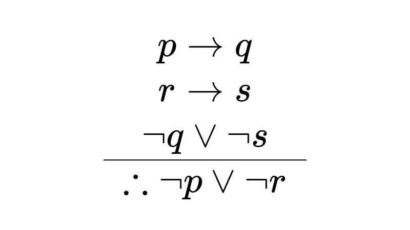
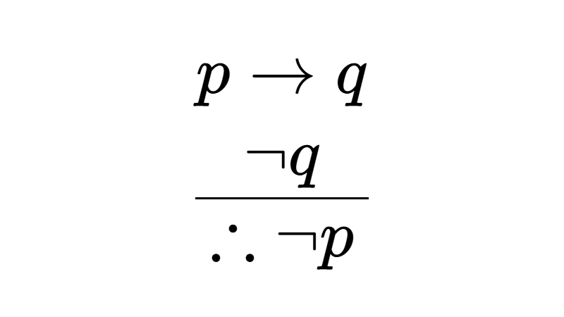
It is important not to confuse the constructive dilemma with the destructive dilemma, as they operate under opposite deductive mechanisms. While the constructive dilemma works as an extension of modus ponens by affirming antecedents to conclude the disjunction of their consequents, the destructive dilemma is based on modus tollens.

In the destructive dilemma, one starts with the disjunctive negation of the consequents ¬q ∨ ¬s alongside the two implications, validly deducing the disjunctive negation of the antecedents ¬p ∨ ¬r. Both patterns represent the two canonical ways to process disjunctions through conditional statements in propositional calculus.

Examples

To understand how the law of constructive dilemma operates across diverse contexts, we analyze below five practical scenarios ranging from everyday decisions to algebraic and analytical properties.

Example 1

Premise 1: If it rains this afternoon, we will go see a movie at the cinema (p → q).
Premise 2: If it is sunny this afternoon, we will go for a walk in the park (r → s).
Premise 3: This afternoon it will rain or it will be sunny (p ∨ r).
Conclusion: Therefore, we will go see a movie at the cinema or we will go for a walk in the park (q ∨ s).

In this first case, we have two conditional plans tied to the weather. Upon confirming that one of the two initial weather conditions will occur, we immediately deduce that we will carry out one of the two planned activities.

Example 2

Premise 1: If we are awarded the full scholarship, we will attend the semester at the public university (p → q).
Premise 2: If we get a part-time job, we will pay tuition at the private college (r → s).
Premise 3: We are awarded the full scholarship or we get a part-time job (p ∨ r).
Conclusion: Therefore, we will attend the semester at the public university or we will pay tuition at the private college (q ∨ s).

Here we evaluate two independent paths of educational funding. Because we guarantee that at least one of the two opportunities will be fulfilled, the conclusion reliably preserves the realization of one of the two academic goals.

Example 3

Premise 1: If the package is sent via standard mail, the customer receives it in five business days (p → q).
Premise 2: If the package is sent via express shipping, the customer receives it in twenty-four hours (r → s).
Premise 3: The package is sent via standard mail or via express shipping (p ∨ r).
Conclusion: Therefore, the customer receives it in five business days or receives it in twenty-four hours (q ∨ s).

In this logistical situation, the shipping conditions determine the product delivery times. Since one of the two dispatch options must be selected, we ensure that the final timeframe will match one of the two specified periods.

Example 4

Premise 1: If we evaluate the function f(x) = cos(x), the graph exhibits symmetry with respect to the y-axis (p → q).
Premise 2: If we evaluate the function g(x) = sin(x), the graph exhibits symmetry with respect to the origin (r → s).
Premise 3: We evaluate the function f(x) = cos(x) or we evaluate the function g(x) = sin(x) (p ∨ r).
Conclusion: Therefore, the graph exhibits symmetry with respect to the y-axis or exhibits symmetry with respect to the origin (q ∨ s).

In this mathematical analysis scenario, each trigonometric function under consideration has a well-defined parity behavior. Knowing with certainty that we are working with either the cosine function or the sine function allows us to infer that the resulting curve will exhibit either even symmetry or odd symmetry.

Example 5

Premise 1: If an integer n is a multiple of 4, then n is an even integer (p → q).
Premise 2: If the last digit of the integer n is 0, then n is divisible by 5 (r → s).
Premise 3: The integer n is a multiple of 4 or its last digit is 0 (p ∨ r).
Conclusion: Therefore, the integer n is an even integer or is divisible by 5 (q ∨ s).

Within elementary arithmetic, we link two distinct divisibility properties through their hypotheses. When one of the conditions regarding the structure of the number n is verified, we validly guarantee that the number will satisfy at least one of the two resulting characteristics.

Formal Proof

To verify the logical validity of the constructive dilemma without resorting to excessively lengthy procedures, we can perform a step-by-step deductive proof using laws of logical equivalence and elementary inference rules.

Our goal is to derive the conclusion q ∨ s from the set of initial premises:

1. p → q (Premise 1)
2. r → s (Premise 2)
3. p ∨ r (Premise 3)

First, we apply the proof by cases method to the disjunction in Premise 3, analyzing what occurs when we assume the truth of each of the two alternatives independently.

For the first case, we temporarily assume that the antecedent p is true:

4. p (Case 1 assumption)
5. q (Modus ponens from 1 and 4)
6. q ∨ s (Rule of addition applied to 5)

For the second case, we assume that the second antecedent r is the one that is true:

7. r (Case 2 assumption)
8. s (Modus ponens from 2 and 7)
9. q ∨ s (Rule of addition applied to 8)

Since both assumptions inevitably lead to the same compound statement q ∨ s, we complete the elimination of the initial disjunction (Premise 3) to conclude definitively:

10. q ∨ s (Disjunction elimination rule from 3, 4–6, and 7–9)

In this way, it is formally proved that the conclusion follows with absolute logical necessity from the given premises.

It is worth noting that the validity of this schema can also be verified using a truth table for the associated conditional [(p → q) ∧ (r → s) ∧ (p ∨ r)] → (q ∨ s). However, because it involves four simple propositional variables (p, q, r, and s), that procedure would require constructing and evaluating 2⁴ = 16 rows to confirm that the result is a tautology.

Simple Constructive Dilemma

The simple constructive dilemma is a particular case of this inference rule where both implications lead to the same consequence. Unlike the complex variant, where two distinct outcomes are derived in a disjunction, here the final outcome is reduced to a single proposition.

In this deductive schema, we have two alternative hypotheses or antecedents in the disjunctive premise p ∨ r. However, because both p and r independently imply the same consequent q, the occurrence of either guarantees the inescapable truth of q.

In propositional calculus, the associated conditional for this law is expressed as follows:

[(p → q) ∧ (r → q) ∧ (p ∨ r)] → q

In vertically structured formal deductions, we arrange the three premises above the deduction line:

$$ \begin{array}{cl} p \rightarrow q \\ r \rightarrow q \\ p \lor r \\ \hline \therefore q \end{array} $$

The algebraic foundation of this simplification lies in the idempotence law of disjunction. Applying the standard constructive dilemma formally yields the intermediate conclusion q ∨ q, which is logically equivalent to q (that is, q ∨ q ≡ q).

Example 1

Premise 1: If we take the highway route, we will arrive on time for the conference (p → q).
Premise 2: If we take the shortcut via the main avenue, we will arrive on time for the conference (r → q).
Premise 3: We take the highway route or we take the shortcut via the main avenue (p ∨ r).
Conclusion: Therefore, we will arrive on time for the conference (q).

In this everyday example, we have two different travel routes leading to a common outcome. Since we must travel along one of the two routes, we reliably ensure that we will arrive on time at our destination, regardless of which alternative is taken.

Example 2

Premise 1: If the real number x is strictly positive (x > 0), then its square is positive: x² > 0 (p → q).
Premise 2: If the real number x is strictly negative (x < 0), then its square is positive: x² > 0 (r → q).
Premise 3: The non-zero real number x is strictly positive or strictly negative (p ∨ r).
Conclusion: Therefore, the square of the non-zero real number x is positive: x² > 0 (q).

In this algebraic analysis, we evaluate the sign of a non-zero real number via a disjunctive partition. Since both sign conditions lead to the same property for the squared power, we conclude the positivity of the final result with complete rigor.